math.scad
Assorted math functions, including linear interpolation, list operations (sums, mean, products), convolution, quantization, log2, hyperbolic trig functions, random numbers, derivatives, polynomials, and root finding.
To use, add the following lines to the beginning of your file:
include <BOSL2/std.scad>
-
Section: Miscellaneous Functions
-
sqr()– Returns the square of the given value. -
log2()– Returns the log base 2 of the given value. -
hypot()– Returns the hypotenuse length of a 2D or 3D triangle. -
factorial()– Returns the factorial of the given integer. -
binomial()– Returns the binomial coefficients of the integern. -
binomial_coefficient()– Returns thek-th binomial coefficient of the integern. -
gcd()– Returns the Greatest Common Divisor/Factor of two integers. -
lcm()– Returns the Least Common Multiple of two or more integers.
-
-
Section: Hyperbolic Trigonometry
-
sinh()– Returns the hyperbolic sine of the given value. -
cosh()– Returns the hyperbolic cosine of the given value. -
tanh()– Returns the hyperbolic tangent of the given value. -
asinh()– Returns the hyperbolic arc-sine of the given value. -
acosh()– Returns the hyperbolic arc-cosine of the given value. -
atanh()– Returns the hyperbolic arc-tangent of the given value.
-
-
Section: Constraints and Modulos
-
constrain()– Returns a value constrained betweenminvalandmaxval, inclusive. -
posmod()– Returns the positive modulo of a value. -
modang()– Returns an angle normalized to between -180º and 180º.
-
-
Section: Operations on Lists (Sums, Mean, Products)
-
sum()– Returns the sum of a list of values. -
mean()– Returns the mean value of a list of values. -
median()– Returns the median value of a list of values. -
deltas()– Returns the deltas between a list of values. -
cumsum()– Returns the running cumulative sum of a list of values. -
product()– Returns the multiplicative product of a list of values. -
cumprod()– Returns the running cumulative product of a list of values. -
convolve()– Returns the convolution ofpandq. -
sum_of_sines()– Returns the sum of one or more sine waves at a given angle.
-
-
Section: Random Number Generation
-
rand_int()– Returns a random integer. -
random_points()– Returns a list of random points. -
gaussian_rands()– Returns a list of random numbers with a gaussian distribution. -
exponential_rands()– Returns a list of random numbers with an exponential distribution. -
spherical_random_points()– Returns a list of random points on the surface of a sphere. -
random_polygon()– Returns the CCW path of a simple random polygon.
-
-
-
complex()– Replaces scalars in a list or matrix with complex number 2-vectors. -
c_mul()– Multiplies two complex numbers. -
c_div()– Divides two complex numbers. -
c_conj()– Returns the complex conjugate of the input. -
c_real()– Returns the real part of a complex number, vector or matrix.. -
c_imag()– Returns the imaginary part of a complex number, vector or matrix.. -
c_ident()– Returns an n by n complex identity matrix. -
c_norm()– Returns the norm of a complex number or vector.
-
-
-
quadratic_roots()– Computes roots for the quadratic equation. -
polynomial()– Calculates a polynomial equation at a given value. -
poly_mult()– Returns the polynomial result of multiplying two polynomial equations. -
poly_div()– Returns the polynomial quotient and remainder results of dividing two polynomial equations. -
poly_add()– Returns the polynomial sum of adding two polynomial equations. -
poly_roots()– Returns all complex number roots of the given real polynomial. -
real_roots()– Returns all real roots of the given real polynomial.
-
-
Section: Operations on Functions
-
root_find()– Finds a root of the given continuous function.
-
Synopsis: The golden ratio φ (phi). Approximately 1.6180339887
Description:
The golden ratio φ (phi). Approximately 1.6180339887
Synopsis: A tiny value to compare floating point values. 1e-9
Description:
A really small value useful in comparing floating point numbers. ie: abs(a-b)<EPSILON 1e-9
Synopsis: The floating point value for Infinite.
Description:
The value inf, useful for comparisons.
Synopsis: The floating point value for Not a Number.
Description:
The value nan, useful for comparisons.
Synopsis: Creates a list of incrementing numbers.
See Also: idx()
Usage:
- list = count(n, [s], [step], [reverse]);
Description:
Creates a list of n numbers, starting at s, incrementing by step each time.
You can also pass a list for n and then the length of the input list is used.
Arguments:
| By Position | What it does |
|---|---|
n |
The length of the list of numbers to create, or a list to match the length of |
s |
The starting value of the list of numbers. |
step |
The amount to increment successive numbers in the list. |
reverse |
Reverse the list. Default: false. |
Example 1:
include <BOSL2/std.scad>
nl1 = count(5);  // Returns: [0,1,2,3,4]
nl2 = count(5,3);  // Returns: [3,4,5,6,7]
nl3 = count(4,3,2);  // Returns: [3,5,7,9]
nl4 = count(5,reverse=true);    // Returns: [4,3,2,1,0]
nl5 = count(5,3,reverse=true);  // Returns: [7,6,5,4,3]
Synopsis: Linearly interpolates between two values.
Topics: Interpolation, Math
See Also: v_lookup(), lerpn()
Usage:
- x = lerp(a, b, u);
- l = lerp(a, b, LIST);
Description:
Interpolate between two values or vectors.
If u is given as a number, returns the single interpolated value.
If u is 0.0, then the value of a is returned.
If u is 1.0, then the value of b is returned.
If u is a range, or list of numbers, returns a list of interpolated values.
It is valid to use a u value outside the range 0 to 1. The result will be an extrapolation
along the slope formed by a and b.
Arguments:
| By Position | What it does |
|---|---|
a |
First value or vector. |
b |
Second value or vector. |
u |
The proportion from a to b to calculate. Standard range is 0.0 to 1.0, inclusive. If given as a list or range of values, returns a list of results. |
Example 1:
include <BOSL2/std.scad>
x = lerp(0,20,0.3);  // Returns: 6
x = lerp(0,20,0.8);  // Returns: 16
x = lerp(0,20,-0.1); // Returns: -2
x = lerp(0,20,1.1);  // Returns: 22
p = lerp([0,0],[20,10],0.25);  // Returns [5,2.5]
l = lerp(0,20,[0.4,0.6]);  // Returns: [8,12]
l = lerp(0,20,[0.25:0.25:0.75]);  // Returns: [5,10,15]
Example 2:
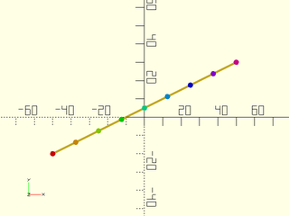
include <BOSL2/std.scad>
p1 = [-50,-20];  p2 = [50,30];
stroke([p1,p2]);
pts = lerp(p1, p2, [0:1/8:1]);
// Points colored in ROYGBIV order.
rainbow(pts) translate($item) circle(d=3,$fn=8);
Synopsis: Returns exactly n values, linearly interpolated between a and b.
Topics: Interpolation, Math
See Also: v_lookup(), lerp()
Usage:
- x = lerpn(a, b, n);
- x = lerpn(a, b, n, [endpoint]);
Description:
Returns exactly n values, linearly interpolated between a and b.
If endpoint is true, then the last value will exactly equal b.
If endpoint is false, then the last value will be a+(b-a)*(1-1/n).
Arguments:
| By Position | What it does |
|---|---|
a |
First value or vector. |
b |
Second value or vector. |
n |
The number of values to return. |
endpoint |
If true, the last value will be exactly b. If false, the last value will be one step less. |
Example 1:
include <BOSL2/std.scad>
l = lerpn(-4,4,9);        // Returns: [-4,-3,-2,-1,0,1,2,3,4]
l = lerpn(-4,4,8,false);  // Returns: [-4,-3,-2,-1,0,1,2,3]
l = lerpn(0,1,6);         // Returns: [0, 0.2, 0.4, 0.6, 0.8, 1]
l = lerpn(0,1,5,false);   // Returns: [0, 0.2, 0.4, 0.6, 0.8]
Synopsis: Returns the square of the given value.
Topics: Math
Usage:
- x2 = sqr(x);
Description:
If given a number, returns the square of that number, If given a vector, returns the sum-of-squares/dot product of the vector elements. If given a matrix, returns the matrix multiplication of the matrix with itself.
Example 1:
include <BOSL2/std.scad>
sqr(3);     // Returns: 9
sqr(-4);    // Returns: 16
sqr([2,3,4]); // Returns: 29
sqr([[1,2],[3,4]]);  // Returns [[7,10],[15,22]]
Synopsis: Returns the log base 2 of the given value.
Topics: Math
Usage:
- val = log2(x);
Description:
Returns the logarithm base 2 of the value given.
Example 1:
include <BOSL2/std.scad>
log2(0.125);  // Returns: -3
log2(16);     // Returns: 4
log2(256);    // Returns: 8
Synopsis: Returns the hypotenuse length of a 2D or 3D triangle.
Topics: Math
Usage:
- l = hypot(x, y, [z]);
Description:
Calculate hypotenuse length of a 2D or 3D triangle.
Arguments:
| By Position | What it does |
|---|---|
x |
Length on the X axis. |
y |
Length on the Y axis. |
z |
Length on the Z axis. Optional. |
Example 1:
include <BOSL2/std.scad>
l = hypot(3,4);  // Returns: 5
l = hypot(3,4,5);  // Returns: ~7.0710678119
Synopsis: Returns the factorial of the given integer.
Topics: Math
See Also: hypot(), sqr(), log2()
Usage:
- x = factorial(n, [d]);
Description:
Returns the factorial of the given integer value, or n!/d! if d is given.
Arguments:
| By Position | What it does |
|---|---|
n |
The integer number to get the factorial of. (n!) |
d |
If given, the returned value will be (n! / d!) |
Example 1:
include <BOSL2/std.scad>
x = factorial(4);  // Returns: 24
y = factorial(6);  // Returns: 720
z = factorial(9);  // Returns: 362880
Synopsis: Returns the binomial coefficients of the integer n.
Topics: Math
See Also: hypot(), sqr(), log2(), factorial()
Usage:
- x = binomial(n);
Description:
Returns the binomial coefficients of the integer n.
Arguments:
| By Position | What it does |
|---|---|
n |
The integer to get the binomial coefficients of |
Example 1:
include <BOSL2/std.scad>
x = binomial(3);  // Returns: [1,3,3,1]
y = binomial(4);  // Returns: [1,4,6,4,1]
z = binomial(6);  // Returns: [1,6,15,20,15,6,1]
Synopsis: Returns the k-th binomial coefficient of the integer n.
Topics: Math
See Also: hypot(), sqr(), log2(), factorial()
Usage:
- x = binomial_coefficient(n, k);
Description:
Returns the k-th binomial coefficient of the integer n.
Arguments:
| By Position | What it does |
|---|---|
n |
The integer to get the binomial coefficient of |
k |
The binomial coefficient index |
Example 1:
include <BOSL2/std.scad>
x = binomial_coefficient(3,2);  // Returns: 3
y = binomial_coefficient(10,6); // Returns: 210
Synopsis: Returns the Greatest Common Divisor/Factor of two integers.
Topics: Math
See Also: hypot(), sqr(), log2(), factorial(), binomial(), lcm()
Usage:
- x = gcd(a,b)
Description:
Computes the Greatest Common Divisor/Factor of a and b.
Synopsis: Returns the Least Common Multiple of two or more integers.
Topics: Math
See Also: hypot(), sqr(), log2(), factorial(), binomial(), gcd()
Usage:
- div = lcm(a, b);
- divs = lcm(list);
Description:
Computes the Least Common Multiple of the two arguments or a list of arguments. Inputs should be non-zero integers. The output is always a positive integer. It is an error to pass zero as an argument.
Synopsis: Returns the hyperbolic sine of the given value.
Topics: Math, Trigonometry
See Also: cosh(), tanh(), asinh(), acosh(), atanh()
Usage:
- a = sinh(x);
Description:
Takes a value x, and returns the hyperbolic sine of it.
Synopsis: Returns the hyperbolic cosine of the given value.
Topics: Math, Trigonometry
See Also: sinh(), tanh(), asinh(), acosh(), atanh()
Usage:
- a = cosh(x);
Description:
Takes a value x, and returns the hyperbolic cosine of it.
Synopsis: Returns the hyperbolic tangent of the given value.
Topics: Math, Trigonometry
See Also: sinh(), cosh(), asinh(), acosh(), atanh()
Usage:
- a = tanh(x);
Description:
Takes a value x, and returns the hyperbolic tangent of it.
Synopsis: Returns the hyperbolic arc-sine of the given value.
Topics: Math, Trigonometry
See Also: sinh(), cosh(), tanh(), acosh(), atanh()
Usage:
- a = asinh(x);
Description:
Takes a value x, and returns the inverse hyperbolic sine of it.
Synopsis: Returns the hyperbolic arc-cosine of the given value.
Topics: Math, Trigonometry
See Also: sinh(), cosh(), tanh(), asinh(), atanh()
Usage:
- a = acosh(x);
Description:
Takes a value x, and returns the inverse hyperbolic cosine of it.
Synopsis: Returns the hyperbolic arc-tangent of the given value.
Topics: Math, Trigonometry
See Also: sinh(), cosh(), tanh(), asinh(), acosh()
Usage:
- a = atanh(x);
Description:
Takes a value x, and returns the inverse hyperbolic tangent of it.
Synopsis: Returns x quantized to the nearest integer multiple of y.
Topics: Math, Quantization
See Also: quantdn(), quantup()
Usage:
- num = quant(x, y);
Description:
Quantize a value x to an integer multiple of y, rounding to the nearest multiple.
The value of y does NOT have to be an integer. If x is a list, then every item
in that list will be recursively quantized.
Arguments:
| By Position | What it does |
|---|---|
x |
The value or list to quantize. |
y |
Positive quantum to quantize to |
Example 1:
include <BOSL2/std.scad>
a = quant(12,4);    // Returns: 12
b = quant(13,4);    // Returns: 12
c = quant(13.1,4);  // Returns: 12
d = quant(14,4);    // Returns: 16
e = quant(14.1,4);  // Returns: 16
f = quant(15,4);    // Returns: 16
g = quant(16,4);    // Returns: 16
h = quant(9,3);     // Returns: 9
i = quant(10,3);    // Returns: 9
j = quant(10.4,3);  // Returns: 9
k = quant(10.5,3);  // Returns: 12
l = quant(11,3);    // Returns: 12
m = quant(12,3);    // Returns: 12
n = quant(11,2.5);  // Returns: 10
o = quant(12,2.5);  // Returns: 12.5
p = quant([12,13,13.1,14,14.1,15,16],4);  // Returns: [12,12,12,16,16,16,16]
q = quant([9,10,10.4,10.5,11,12],3);      // Returns: [9,9,9,12,12,12]
r = quant([[9,10,10.4],[10.5,11,12]],3);  // Returns: [[9,9,9],[12,12,12]]
Synopsis: Returns x quantized down to an integer multiple of y.
Topics: Math, Quantization
Usage:
- num = quantdn(x, y);
Description:
Quantize a value x to an integer multiple of y, rounding down to the previous multiple.
The value of y does NOT have to be an integer. If x is a list, then every item in that
list will be recursively quantized down.
Arguments:
| By Position | What it does |
|---|---|
x |
The value or list to quantize. |
y |
Postive quantum to quantize to. |
Example 1:
include <BOSL2/std.scad>
a = quantdn(12,4);    // Returns: 12
b = quantdn(13,4);    // Returns: 12
c = quantdn(13.1,4);  // Returns: 12
d = quantdn(14,4);    // Returns: 12
e = quantdn(14.1,4);  // Returns: 12
f = quantdn(15,4);    // Returns: 12
g = quantdn(16,4);    // Returns: 16
h = quantdn(9,3);     // Returns: 9
i = quantdn(10,3);    // Returns: 9
j = quantdn(10.4,3);  // Returns: 9
k = quantdn(10.5,3);  // Returns: 9
l = quantdn(11,3);    // Returns: 9
m = quantdn(12,3);    // Returns: 12
n = quantdn(11,2.5);  // Returns: 10
o = quantdn(12,2.5);  // Returns: 10
p = quantdn([12,13,13.1,14,14.1,15,16],4);  // Returns: [12,12,12,12,12,12,16]
q = quantdn([9,10,10.4,10.5,11,12],3);      // Returns: [9,9,9,9,9,12]
r = quantdn([[9,10,10.4],[10.5,11,12]],3);  // Returns: [[9,9,9],[9,9,12]]
Synopsis: Returns x quantized uo to an integer multiple of y.
Topics: Math, Quantization
Usage:
- num = quantup(x, y);
Description:
Quantize a value x to an integer multiple of y, rounding up to the next multiple.
The value of y does NOT have to be an integer. If x is a list, then every item in
that list will be recursively quantized up.
Arguments:
| By Position | What it does |
|---|---|
x |
The value or list to quantize. |
y |
Positive quantum to quantize to. |
Example 1:
include <BOSL2/std.scad>
a = quantup(12,4);    // Returns: 12
b = quantup(13,4);    // Returns: 16
c = quantup(13.1,4);  // Returns: 16
d = quantup(14,4);    // Returns: 16
e = quantup(14.1,4);  // Returns: 16
f = quantup(15,4);    // Returns: 16
g = quantup(16,4);    // Returns: 16
h = quantup(9,3);     // Returns: 9
i = quantup(10,3);    // Returns: 12
j = quantup(10.4,3);  // Returns: 12
k = quantup(10.5,3);  // Returns: 12
l = quantup(11,3);    // Returns: 12
m = quantup(12,3);    // Returns: 12
n = quantdn(11,2.5);  // Returns: 12.5
o = quantdn(12,2.5);  // Returns: 12.5
p = quantup([12,13,13.1,14,14.1,15,16],4);  // Returns: [12,16,16,16,16,16,16]
q = quantup([9,10,10.4,10.5,11,12],3);      // Returns: [9,12,12,12,12,12]
r = quantup([[9,10,10.4],[10.5,11,12]],3);  // Returns: [[9,12,12],[12,12,12]]
Synopsis: Returns a value constrained between minval and maxval, inclusive.
Topics: Math
Usage:
- val = constrain(v, minval, maxval);
Description:
Constrains value to a range of values between minval and maxval, inclusive.
Arguments:
| By Position | What it does |
|---|---|
v |
value to constrain. |
minval |
minimum value to return, if out of range. |
maxval |
maximum value to return, if out of range. |
Example 1:
include <BOSL2/std.scad>
a = constrain(-5, -1, 1);   // Returns: -1
b = constrain(5, -1, 1);    // Returns: 1
c = constrain(0.3, -1, 1);  // Returns: 0.3
d = constrain(9.1, 0, 9);   // Returns: 9
e = constrain(-0.1, 0, 9);  // Returns: 0
Synopsis: Returns the positive modulo of a value.
Topics: Math
See Also: constrain(), modang()
Usage:
- mod = posmod(x, m)
Description:
Returns the positive modulo m of x. Value returned will be in the range 0 ... m-1.
Arguments:
| By Position | What it does |
|---|---|
x |
The value to constrain. |
m |
Modulo value. |
Example 1:
include <BOSL2/std.scad>
a = posmod(-700,360);  // Returns: 340
b = posmod(-270,360);  // Returns: 90
c = posmod(-120,360);  // Returns: 240
d = posmod(120,360);   // Returns: 120
e = posmod(270,360);   // Returns: 270
f = posmod(700,360);   // Returns: 340
g = posmod(3,2.5);     // Returns: 0.5
Synopsis: Returns an angle normalized to between -180º and 180º.
Topics: Math
See Also: constrain(), posmod()
Usage:
- ang = modang(x);
Description:
Takes an angle in degrees and normalizes it to an equivalent angle value between -180 and 180.
Example 1:
include <BOSL2/std.scad>
a1 = modang(-700);  // Returns: 20
a2 = modang(-270);  // Returns: 90
a3 = modang(-120);  // Returns: -120
a4 = modang(120);   // Returns: 120
a5 = modang(270);   // Returns: -90
a6 = modang(700);   // Returns: -20
Synopsis: Returns the sum of a list of values.
Topics: Math
See Also: mean(), median(), product(), cumsum()
Usage:
- x = sum(v, [dflt]);
Description:
Returns the sum of all entries in the given consistent list.
If passed an array of vectors, returns the sum the vectors.
If passed an array of matrices, returns the sum of the matrices.
If passed an empty list, the value of dflt will be returned.
Arguments:
| By Position | What it does |
|---|---|
v |
The list to get the sum of. |
dflt |
The default value to return if v is an empty list. Default: 0 |
Example 1:
include <BOSL2/std.scad>
sum([1,2,3]);  // returns 6.
sum([[1,2,3], [3,4,5], [5,6,7]]);  // returns [9, 12, 15]
Synopsis: Returns the mean value of a list of values.
Topics: Math, Statistics
See Also: sum(), median(), product()
Usage:
- x = mean(v);
Description:
Returns the arithmetic mean/average of all entries in the given array. If passed a list of vectors, returns a vector of the mean of each part.
Arguments:
| By Position | What it does |
|---|---|
v |
The list of values to get the mean of. |
Example 1:
include <BOSL2/std.scad>
mean([2,3,4]);  // returns 3.
mean([[1,2,3], [3,4,5], [5,6,7]]);  // returns [3, 4, 5]
Synopsis: Returns the median value of a list of values.
Topics: Math, Statistics
See Also: sum(), mean(), product()
Usage:
- middle = median(v)
Description:
Returns the median of the given vector.
Synopsis: Returns the deltas between a list of values.
Topics: Math, Statistics
See Also: sum(), mean(), median(), product()
Usage:
- delts = deltas(v,[wrap]);
Description:
Returns a list with the deltas of adjacent entries in the given list, optionally wrapping back to the front. The list should be a consistent list of numeric components (numbers, vectors, matrix, etc). Given [a,b,c,d], returns [b-a,c-b,d-c].
Arguments:
| By Position | What it does |
|---|---|
v |
The list to get the deltas of. |
wrap |
If true, wrap back to the start from the end. ie: return the difference between the last and first items as the last delta. Default: false |
Example 1:
include <BOSL2/std.scad>
deltas([2,5,9,17]);  // returns [3,4,8].
deltas([[1,2,3], [3,6,8], [4,8,11]]);  // returns [[2,4,5], [1,2,3]]
Synopsis: Returns the running cumulative sum of a list of values.
Topics: Math, Statistics
See Also: sum(), mean(), median(), product()
Usage:
- sums = cumsum(v);
Description:
Returns a list where each item is the cumulative sum of all items up to and including the corresponding entry in the input list. If passed an array of vectors, returns a list of cumulative vectors sums.
Arguments:
| By Position | What it does |
|---|---|
v |
The list to get the sum of. |
Example 1:
include <BOSL2/std.scad>
cumsum([1,1,1]);  // returns [1,2,3]
cumsum([2,2,2]);  // returns [2,4,6]
cumsum([1,2,3]);  // returns [1,3,6]
cumsum([[1,2,3], [3,4,5], [5,6,7]]);  // returns [[1,2,3], [4,6,8], [9,12,15]]
Synopsis: Returns the multiplicative product of a list of values.
Topics: Math, Statistics
See Also: sum(), mean(), median(), cumsum()
Usage:
- x = product(v);
Description:
Returns the product of all entries in the given list. If passed a list of vectors of same dimension, returns a vector of products of each part. If passed a list of square matrices, returns the resulting product matrix.
Arguments:
| By Position | What it does |
|---|---|
v |
The list to get the product of. |
Example 1:
include <BOSL2/std.scad>
product([2,3,4]);  // returns 24.
product([[1,2,3], [3,4,5], [5,6,7]]);  // returns [15, 48, 105]
Synopsis: Returns the running cumulative product of a list of values.
Topics: Math, Statistics
See Also: sum(), mean(), median(), product(), cumsum()
Usage:
- prod_list = cumprod(list, [right]);
Description:
Returns a list where each item is the cumulative product of all items up to and including the corresponding entry in the input list.
If passed an array of vectors, returns a list of elementwise vector products. If passed a list of square matrices by default returns matrix
products multiplying on the left, so a list [A,B,C] will produce the output [A,BA,CBA]. If you set right=true then it returns
the product of multiplying on the right, so a list [A,B,C] will produce the output [A,AB,ABC] in that case.
Arguments:
| By Position | What it does |
|---|---|
list |
The list to get the cumulative product of. |
right |
if true multiply matrices on the right |
Example 1:
include <BOSL2/std.scad>
cumprod([1,3,5]);  // returns [1,3,15]
cumprod([2,2,2]);  // returns [2,4,8]
cumprod([[1,2,3], [3,4,5], [5,6,7]]));  // returns [[1, 2, 3], [3, 8, 15], [15, 48, 105]]
Synopsis: Returns the convolution of p and q.
Topics: Math, Statistics
See Also: sum(), mean(), median(), product(), cumsum()
Usage:
- x = convolve(p,q);
Description:
Given two vectors, or one vector and a path or two paths of the same dimension, finds the convolution of them. If both parameter are vectors, returns the vector convolution. If one parameter is a vector and the other a path, convolves using products by scalars and returns a path. If both parameters are paths, convolve using scalar products and returns a vector. The returned vector or path has length len(p)+len(q)-1.
Arguments:
| By Position | What it does |
|---|---|
p |
The first vector or path. |
q |
The second vector or path. |
Example 1:
include <BOSL2/std.scad>
a = convolve([1,1],[1,2,1]); // Returns: [1,3,3,1]
b = convolve([1,2,3],[1,2,1])); // Returns: [1,4,8,8,3]
c = convolve([[1,1],[2,2],[3,1]],[1,2,1])); // Returns: [[1,1],[4,4],[8,6],[8,4],[3,1]]
d = convolve([[1,1],[2,2],[3,1]],[[1,2],[2,1]])); // Returns:  [3,9,11,7]
Synopsis: Returns the sum of one or more sine waves at a given angle.
Topics: Math, Statistics
See Also: sum(), mean(), median(), product(), cumsum()
Usage:
- sum_of_sines(a,sines)
Description:
Given a list of sine waves, returns the sum of the sines at the given angle.
Each sine wave is given as an [AMPLITUDE, FREQUENCY, PHASE_ANGLE] triplet.
-
AMPLITUDEis the height of the sine wave above (and below)0. -
FREQUENCYis the number of times the sine wave repeats in 360º. -
PHASE_ANGLEis the offset in degrees of the sine wave.
Arguments:
| By Position | What it does |
|---|---|
a |
Angle to get the value for. |
sines |
List of [amplitude, frequency, phase_angle] items, where the frequency is the number of times the cycle repeats around the circle. |
Example 1:
include <BOSL2/std.scad>
v = sum_of_sines(30, [[10,3,0], [5,5.5,60]]);
Synopsis: Returns a random integer.
Topics: Random
See Also: random_points(), gaussian_rands(), random_polygon(), spherical_random_points(), exponential_rands()
Usage:
- rand_int(minval, maxval, n, [seed]);
Description:
Return a list of random integers in the range of minval to maxval, inclusive.
Arguments:
| By Position | What it does |
|---|---|
minval |
Minimum integer value to return. |
maxval |
Maximum integer value to return. |
N |
Number of random integers to return. |
seed |
If given, sets the random number seed. |
Example 1:
include <BOSL2/std.scad>
ints = rand_int(0,100,3);
int = rand_int(-10,10,1)[0];
Synopsis: Returns a list of random points.
See Also: rand_int(), random_polygon(), spherical_random_points()
Usage:
- points = random_points(n, dim, [scale], [seed]);
Description:
Generate n uniform random points of dimension dim with data ranging from -scale to +scale.
The scale may be a number, in which case the random data lies in a cube,
or a vector with dimension dim, in which case each dimension has its own scale.
Arguments:
| By Position | What it does |
|---|---|
n |
number of points to generate. Default: 1 |
dim |
dimension of the points. Default: 2 |
scale |
the scale of the point coordinates. Default: 1 |
seed |
an optional seed for the random generation. |
Synopsis: Returns a list of random numbers with a gaussian distribution.
Topics: Random, Statistics
See Also: rand_int(), random_points(), random_polygon(), spherical_random_points(), exponential_rands()
Usage:
- arr = gaussian_rands([n],[mean], [cov], [seed]);
Description:
Returns a random number or vector with a Gaussian/normal distribution.
Arguments:
| By Position | What it does |
|---|---|
n |
the number of points to return. Default: 1 |
mean |
The average of the random value (a number or vector). Default: 0 |
cov |
covariance matrix of the random numbers, or variance in the 1D case. Default: 1 |
seed |
If given, sets the random number seed. |
Synopsis: Returns a list of random numbers with an exponential distribution.
Topics: Random, Statistics
See Also: rand_int(), random_points(), gaussian_rands(), random_polygon(), spherical_random_points()
Usage:
- arr = exponential_rands([n], [lambda], [seed])
Description:
Returns random numbers with an exponential distribution with parameter lambda, and hence mean 1/lambda.
Arguments:
| By Position | What it does |
|---|---|
n |
number of points to return. Default: 1 |
lambda |
distribution parameter. The mean will be 1/lambda. Default: 1 |
Synopsis: Returns a list of random points on the surface of a sphere.
See Also: rand_int(), random_points(), gaussian_rands(), random_polygon()
Usage:
- points = spherical_random_points([n], [radius], [seed]);
Description:
Generate n 3D uniformly distributed random points lying on a sphere centered at the origin with radius equal to radius.
Arguments:
| By Position | What it does |
|---|---|
n |
number of points to generate. Default: 1 |
radius |
the sphere radius. Default: 1 |
seed |
an optional seed for the random generation. |
Synopsis: Returns the CCW path of a simple random polygon.
See Also: random_points(), spherical_random_points()
Usage:
- points = random_polygon([n], [size], [seed]);
Description:
Generate the n vertices of a random counter-clockwise simple 2d polygon
inside a circle centered at the origin with radius size.
Arguments:
| By Position | What it does |
|---|---|
n |
number of vertices of the polygon. Default: 3 |
size |
the radius of a circle centered at the origin containing the polygon. Default: 1 |
seed |
an optional seed for the random generation. |
Synopsis: Returns the first derivative estimate of a list of data.
Usage:
- x = deriv(data, [h], [closed])
Description:
Computes a numerical derivative estimate of the data, which may be scalar or vector valued.
The h parameter gives the step size of your sampling so the derivative can be scaled correctly.
If the closed parameter is true the data is assumed to be defined on a loop with data[0] adjacent to
data[len(data)-1]. This function uses a symetric derivative approximation
for internal points, f'(t) = (f(t+h)-f(t-h))/2h. For the endpoints (when closed=false) the algorithm
uses a two point method if sufficient points are available: f'(t) = (3*(f(t+h)-f(t)) - (f(t+2*h)-f(t+h)))/2h.
If h is a vector then it is assumed to be nonuniform, with h[i] giving the sampling distance
between data[i+1] and data[i], and the data values will be linearly resampled at each corner
to produce a uniform spacing for the derivative estimate. At the endpoints a single point method
is used: f'(t) = (f(t+h)-f(t))/h.
Arguments:
| By Position | What it does |
|---|---|
data |
the list of the elements to compute the derivative of. |
h |
the parametric sampling of the data. |
closed |
boolean to indicate if the data set should be wrapped around from the end to the start. |
Synopsis: Returns the second derivative estimate of a list of data.
Usage:
- x = deriv2(data, [h], [closed])
Description:
Computes a numerical estimate of the second derivative of the data, which may be scalar or vector valued.
The h parameter gives the step size of your sampling so the derivative can be scaled correctly.
If the closed parameter is true the data is assumed to be defined on a loop with data[0] adjacent to
data[len(data)-1]. For internal points this function uses the approximation
f''(t) = (f(t-h)-2f(t)+f(t+h))/h^2. For the endpoints (when closed=false),
when sufficient points are available, the method is either the four point expression
f''(t) = (2f(t) - 5f(t+h) + 4f(t+2h) - f(t+3h))/h^2 or
f''(t) = (35f(t) - 104f(t+h) + 114f(t+2h) - 56f(t+3h) + 11f(t+4h)) / 12h^2
if five points are available.
Arguments:
| By Position | What it does |
|---|---|
data |
the list of the elements to compute the derivative of. |
h |
the constant parametric sampling of the data. |
closed |
boolean to indicate if the data set should be wrapped around from the end to the start. |
Synopsis: Returns the third derivative estimate of a list of data.
Usage:
- x = deriv3(data, [h], [closed])
Description:
Computes a numerical third derivative estimate of the data, which may be scalar or vector valued.
The h parameter gives the step size of your sampling so the derivative can be scaled correctly.
If the closed parameter is true the data is assumed to be defined on a loop with data[0] adjacent to
data[len(data)-1]. This function uses a five point derivative estimate, so the input data must include
at least five points:
f'''(t) = (-f(t-2h)+2f(t-h)-2f(t+h)+f(t+2h)) / 2h^3. At the first and second points from the end
the estimates are f'''(t) = (-5f(t)+18f(t+h)-24f(t+2h)+14f(t+3h)-3f(t+4h)) / 2h^3 and
f'''(t) = (-3f(t-h)+10f(t)-12f(t+h)+6f(t+2h)-f(t+3h)) / 2h^3.
Arguments:
| By Position | What it does |
|---|---|
data |
the list of the elements to compute the derivative of. |
h |
the constant parametric sampling of the data. |
closed |
boolean to indicate if the data set should be wrapped around from the end to the start. |
Synopsis: Replaces scalars in a list or matrix with complex number 2-vectors.
Topics: Math, Complex Numbers
See Also: c_mul(), c_div(), c_conj(), c_real(), c_imag(), c_ident(), c_norm()
Usage:
- z = complex(list)
Description:
Converts a real valued number, vector or matrix into its complex analog by replacing all entries with a 2-vector that has zero imaginary part.
Synopsis: Multiplies two complex numbers.
Topics: Math, Complex Numbers
See Also: complex(), c_div(), c_conj(), c_real(), c_imag(), c_ident(), c_norm()
Usage:
- c = c_mul(z1,z2)
Description:
Multiplies two complex numbers, vectors or matrices, where complex numbers or entries are represented as vectors: [REAL, IMAGINARY]. Note that all entries in both arguments must be complex.
Arguments:
| By Position | What it does |
|---|---|
z1 |
First complex number, vector or matrix |
z2 |
Second complex number, vector or matrix |
Synopsis: Divides two complex numbers.
Topics: Math, Complex Numbers
See Also: complex(), c_mul(), c_conj(), c_real(), c_imag(), c_ident(), c_norm()
Usage:
- x = c_div(z1,z2)
Description:
Divides two complex numbers represented by 2D vectors. Returns a complex number as a 2D vector [REAL, IMAGINARY].
Arguments:
| By Position | What it does |
|---|---|
z1 |
First complex number, given as a 2D vector [REAL, IMAGINARY] |
z2 |
Second complex number, given as a 2D vector [REAL, IMAGINARY] |
Synopsis: Returns the complex conjugate of the input.
Topics: Math, Complex Numbers
See Also: complex(), c_mul(), c_div(), c_real(), c_imag(), c_ident(), c_norm()
Usage:
- w = c_conj(z)
Description:
Computes the complex conjugate of the input, which can be a complex number, complex vector or complex matrix.
Synopsis: Returns the real part of a complex number, vector or matrix..
Topics: Math, Complex Numbers
See Also: complex(), c_mul(), c_div(), c_conj(), c_imag(), c_ident(), c_norm()
Usage:
- x = c_real(z)
Description:
Returns real part of a complex number, vector or matrix.
Synopsis: Returns the imaginary part of a complex number, vector or matrix..
Topics: Math, Complex Numbers
See Also: complex(), c_mul(), c_div(), c_conj(), c_real(), c_ident(), c_norm()
Usage:
- x = c_imag(z)
Description:
Returns imaginary part of a complex number, vector or matrix.
Synopsis: Returns an n by n complex identity matrix.
Topics: Math, Complex Numbers
See Also: complex(), c_mul(), c_div(), c_conj(), c_real(), c_imag(), c_norm()
Usage:
- I = c_ident(n)
Description:
Produce an n by n complex identity matrix
Synopsis: Returns the norm of a complex number or vector.
Topics: Math, Complex Numbers
See Also: complex(), c_mul(), c_div(), c_conj(), c_real(), c_imag(), c_ident()
Usage:
- n = c_norm(z)
Description:
Compute the norm of a complex number or vector.
Synopsis: Computes roots for the quadratic equation.
Topics: Math, Geometry, Complex Numbers
See Also: polynomial(), poly_mult(), poly_div(), poly_add()
Usage:
- roots = quadratic_roots(a, b, c, [real])
Description:
Computes roots of the quadratic equation ax^2+bx+c==0, where the coefficients are real numbers. If real is true then returns only the real roots. Otherwise returns a pair of complex values. This method may be more reliable than the general root finder at distinguishing real roots from complex roots. Algorithm from: https://people.csail.mit.edu/bkph/articles/Quadratics.pdf
Synopsis: Calculates a polynomial equation at a given value.
Topics: Math, Complex Numbers
See Also: quadratic_roots(), poly_mult(), poly_div(), poly_add(), poly_roots()
Usage:
- x = polynomial(p, z)
Description:
Evaluates specified real polynomial, p, at the complex or real input value, z.
The polynomial is specified as p=[a_n, a_{n-1},...,a_1,a_0]
where a_n is the z^n coefficient. Polynomial coefficients are real.
The result is a number if z is a number and a complex number otherwise.
Synopsis: Returns the polynomial result of multiplying two polynomial equations.
Topics: Math
See Also: quadratic_roots(), polynomial(), poly_div(), poly_add(), poly_roots()
Usage:
- x = polymult(p,q)
- x = polymult([p1,p2,p3,...])
Description:
Given a list of polynomials represented as real algebraic coefficient lists, with the highest degree coefficient first, computes the coefficient list of the product polynomial.
Synopsis: Returns the polynomial quotient and remainder results of dividing two polynomial equations.
Topics: Math
See Also: quadratic_roots(), polynomial(), poly_mult(), poly_add(), poly_roots()
Usage:
- [quotient,remainder] = poly_div(n,d)
Description:
Computes division of the numerator polynomial by the denominator polynomial and returns a list of two polynomials, [quotient, remainder]. If the division has no remainder then the zero polynomial [0] is returned for the remainder. Similarly if the quotient is zero the returned quotient will be [0].
Synopsis: Returns the polynomial sum of adding two polynomial equations.
Topics: Math
See Also: quadratic_roots(), polynomial(), poly_mult(), poly_div(), poly_roots()
Usage:
- sum = poly_add(p,q)
Description:
Computes the sum of two polynomials.
Synopsis: Returns all complex number roots of the given real polynomial.
Topics: Math, Complex Numbers
See Also: quadratic_roots(), polynomial(), poly_mult(), poly_div(), poly_add()
Usage:
- roots = poly_roots(p, [tol]);
Description:
Returns all complex roots of the specified real polynomial p. The polynomial is specified as p=[a_n, a_{n-1},...,a_1,a_0] where a_n is the z^n coefficient. The tol parameter gives the stopping tolerance for the iteration. The polynomial must have at least one non-zero coefficient. Convergence is poor if the polynomial has any repeated roots other than zero.
Arguments:
| By Position | What it does |
|---|---|
p |
polynomial coefficients with higest power coefficient first |
tol |
tolerance for iteration. Default: 1e-14 |
Synopsis: Returns all real roots of the given real polynomial.
Topics: Math, Complex Numbers
See Also: quadratic_roots(), polynomial(), poly_mult(), poly_div(), poly_add(), poly_roots()
Usage:
- roots = real_roots(p, [eps], [tol])
Description:
Returns the real roots of the specified real polynomial p. The polynomial is specified as p=[a_n, a_{n-1},...,a_1,a_0] where a_n is the x^n coefficient. This function works by computing the complex roots and returning those roots where the imaginary part is closed to zero. By default it uses a computed error bound from the polynomial solver to decide whether imaginary parts are zero. You can specify eps, in which case the test is z.y/(1+norm(z)) < eps. Because of poor convergence and higher error for repeated roots, such roots may be missed by the algorithm because their imaginary part is large.
Arguments:
| By Position | What it does |
|---|---|
p |
polynomial to solve as coefficient list, highest power term first |
eps |
used to determine whether imaginary parts of roots are zero |
tol |
tolerance for the complex polynomial root finder |
Synopsis: Finds a root of the given continuous function.
Topics: Math
See Also: quadratic_roots(), polynomial(), poly_mult(), poly_div(), poly_add(), poly_roots()
Usage:
- x = root_find(f, x0, x1, [tol])
Description:
Find a root of the continuous function f where the sign of f(x0) is different from the sign of f(x1). The function f is a function literal accepting one argument. You must have a version of OpenSCAD that supports function literals (2021.01 or newer). The tolerance (tol) specifies the accuracy of the solution: abs(f(x)) < tol * yrange, where yrange is the range of observed function values. This function can only find roots that cross the x axis: it cannot find the the root of x^2.
Arguments:
| By Position | What it does |
|---|---|
f |
function literal for a scalar-valued single variable function |
x0 |
endpoint of interval to search for root |
x1 |
second endpoint of interval to search for root |
tol |
tolerance for solution. Default: 1e-15 |