skin.scad
This file provides functions and modules that construct shapes from a list of cross sections. In the case of skin() you specify each cross sectional shape yourself, and the number of points can vary. The various forms of sweep use a fixed shape, which may follow a path, or be transformed in other ways to produce the list of cross sections. In all cases it is the user's responsibility to avoid creating a self-intersecting shape, which will produce cryptic CGAL errors. This file was inspired by list-comprehension-demos skin():
To use, add the following lines to the beginning of your file:
include <BOSL2/std.scad>
-
-
skin()– Connect a sequence of arbitrary polygons into a 3D object. [VNF] [Geom] -
linear_sweep()– Create a linear extrusion from a path, with optional texturing. [VNF] [Geom] -
rotate_sweep()– Create a surface of revolution from a path with optional texturing. [VNF] [Geom] -
spiral_sweep()– Sweep a path along a helix. [VNF] [Geom] -
path_sweep()– Sweep a 2d polygon path along a 2d or 3d path. [VNF] [Geom] -
path_sweep2d()– Sweep a 2d polygon path along a 2d path allowing self-intersection. [VNF] [Geom] -
sweep()– Construct a 3d object from arbitrary transformations of a 2d polygon path. [VNF] [Geom]
-
-
Section: Functions for resampling and slicing profile lists
-
subdivide_and_slice()– Resample list of paths to have the same point count and interpolate additional paths. [PathList] -
slice_profiles()– Linearly interpolates between path profiles. [PathList] -
rot_resample()– Resample a list of rotation operators. [MatList] -
associate_vertices()– Create vertex association to control howskin()links vertices. [PathList]
-
-
-
texture()– Produce a standard texture.
-
Synopsis: Connect a sequence of arbitrary polygons into a 3D object. [VNF] [Geom]
See Also: sweep(), linear_sweep(), rotate_sweep(), spiral_sweep(), path_sweep(), offset_sweep()
Usage: As module:
- skin(profiles, slices, [z=], [refine=], [method=], [sampling=], [caps=], [closed=], [style=], [convexity=], [anchor=],[cp=],[spin=],[orient=],[atype=]) [ATTACHMENTS];
Usage: As function:
- vnf = skin(profiles, slices, [z=], [refine=], [method=], [sampling=], [caps=], [closed=], [style=], [anchor=],[cp=],[spin=],[orient=],[atype=]);
Description:
Given a list of two or more path profiles in 3d space, produces faces to skin a surface between
the profiles. Optionally the first and last profiles can have endcaps, or the first and last profiles
can be connected together. Each profile should be roughly planar, but some variation is allowed.
Each profile must rotate in the same clockwise direction. If called as a function, returns a
VNF structure [VERTICES, FACES]. If called as a module, creates a polyhedron
of the skinned profiles.
The profiles can be specified either as a list of 3d curves or they can be specified as
2d curves with heights given in the z parameter. It is your responsibility to ensure
that the resulting polyhedron is free from self-intersections, which would make it invalid
and can result in cryptic CGAL errors upon rendering with a second object present, even though the polyhedron appears
OK during preview or when rendered by itself.
For this operation to be well-defined, the profiles must all have the same vertex count and
we must assume that profiles are aligned so that vertex i links to vertex i on all polygons.
Many interesting cases do not comply with this restriction. Two basic methods can handle
these cases: either subdivide edges (insert additional points along edges)
or duplicate vertcies (insert edges of length 0) so that both polygons have
the same number of points.
Duplicating vertices allows two distinct points in one polygon to connect to a single point
in the other one, creating
triangular faces. You can adjust non-matching polygons yourself
either by resampling them using subdivide_path() or by duplicating vertices using
repeat_entries. It is OK to pass a polygon that has the same vertex repeated, such as
a square with 5 points (two of which are identical), so that it can match up to a pentagon.
Such a combination would create a triangular face at the location of the duplicated vertex.
Alternatively, skin provides methods (described below) for inserting additional vertices
automatically to make incompatible paths match.
In order for skinned surfaces to look good it is usually necessary to use a fine sampling of
points on all of the profiles, and a large number of extra interpolated slices between the
profiles that you specify. It is generally best if the triangles forming your polyhedron
are approximately equilateral. The slices parameter specifies the number of slices to insert
between each pair of profiles, either a scalar to insert the same number everywhere, or a vector
to insert a different number between each pair.
Resampling may occur, depending on the method parameter, to make profiles compatible.
To force (possibly additional) resampling of the profiles to increase the point density you can set refine=N, which
will multiply the number of points on your profile by N. You can choose between two resampling
schemes using the sampling option, which you can set to "length" or "segment".
The length resampling method resamples proportional to length.
The segment method divides each segment of a profile into the same number of points.
This means that if you refine a profile with the "segment" method you will get N points
on each edge, but if you refine a profile with the "length" method you will get new points
distributed around the profile based on length, so small segments will get fewer new points than longer ones.
A uniform division may be impossible, in which case the code computes an approximation, which may result
in arbitrary distribution of extra points. See subdivide_path() for more details.
Note that when dealing with continuous curves it is always better to adjust the
sampling in your code to generate the desired sampling rather than using the refine argument.
You can choose from five methods for specifying alignment for incommensurate profiles.
The available methods are "distance", "fast_distance", "tangent", "direct" and "reindex".
It is useful to distinguish between continuous curves like a circle and discrete profiles
like a hexagon or star, because the algorithms' suitability depend on this distinction.
The default method for aligning profiles is method="direct".
If you simply supply a list of compatible profiles it will link them up
exactly as you have provided them. You may find that profiles you want to connect define the
right shapes but the point lists don't start from points that you want aligned in your skinned
polyhedron. You can correct this yourself using reindex_polygon, or you can use the "reindex"
method which will look for the index choice that will minimize the length of all of the edges
in the polyhedron—it will produce the least twisted possible result. This algorithm has quadratic
run time so it can be slow with very large profiles.
When the profiles are incommensurate, the "direct" and "reindex" resample them to match. As noted above,
for continuous input curves, it is better to generate your curves directly at the desired sample size,
but for mapping between a discrete profile like a hexagon and a circle, the hexagon must be resampled
to match the circle. When you use "direct" or "reindex" the default sampling value is
of sampling="length" to approximate a uniform length sampling of the profile. This will generally
produce the natural result for connecting two continuously sampled profiles or a continuous
profile and a polygonal one. However depending on your particular case,
sampling="segment" may produce a more pleasing result. These two approaches differ only when
the segments of your input profiles have unequal length.
The "distance", "fast_distance" and "tangent" methods work by duplicating vertices to create
triangular faces. In the skined object created by two polygons, every vertex of a polygon must
have an edge that connects to some vertex on the other one. If you connect two squares this can be
accomplished with four edges, but if you want to connect a square to a pentagon you must add a
fifth edge for the "extra" vertex on the pentagon. You must now decide which vertex on the square to
connect the "extra" edge to. How do you decide where to put that fifth edge? The "distance" method answers this
question by using an optimization: it minimizes the total length of all the edges connecting
the two polygons. This algorithm generally produces a good result when both profiles are discrete ones with
a small number of vertices. It is computationally intensive (O(N^3)) and may be
slow on large inputs. The resulting surfaces generally have curved faces, so be
sure to select a sufficiently large value for slices and refine. Note that for
this method, sampling must be set to "segment", and hence this is the default setting.
Using sampling by length would ignore the repeated vertices and ruin the alignment.
The "fast_distance" method restricts the optimization by assuming that an edge should connect
vertex 0 of the two polygons. This reduces the run time to O(N^2) and makes
the method usable on profiles with more points if you take care to index the inputs to match.
The "tangent" method generally produces good results when
connecting a discrete polygon to a convex, finely sampled curve. Given a polygon and a curve, consider one edge
on the polygon. Find a plane passing through the edge that is tangent to the curve. The endpoints of the edge and
the point of tangency define a triangular face in the output polyhedron. If you work your way around the polygon
edges, you can establish a series of triangular faces in this way, with edges linking the polygon to the curve.
You can then complete the edge assignment by connecting all the edges in between the triangular faces together,
with many edges meeting at each polygon vertex. The result is an alternation of flat triangular faces with conical
curves joining them. Another way to think about it is that it splits the points on the curve up into groups and
connects all the points in one group to the same vertex on the polygon.
The "tangent" method may fail if the curved profile is non-convex, or doesn't have enough points to distinguish
all of the tangent points from each other. The algorithm treats whichever input profile has fewer points as the polygon
and the other one as the curve. Using refine with this method will have little effect on the model, so
you should do it only for agreement with other profiles, and these models are linear, so extra slices also
have no effect. For best efficiency set refine=1 and slices=0. As with the "distance" method, refinement
must be done using the "segment" sampling scheme to preserve alignment across duplicated points.
Note that the "tangent" method produces similar results to the "distance" method on curved inputs. If this
method fails due to concavity, "fast_distance" may be a good option.
It is possible to specify method and refine as arrays, but it is important to observe
matching rules when you do this. If a pair of profiles is connected using "tangent" or "distance"
then the refine values for those two profiles must be equal. If a profile is connected by
a vertex duplicating method on one side and a resampling method on the other side, then
refine must be set so that the resulting number of vertices matches the number that is
used for the resampled profiles. The best way to avoid confusion is to ensure that the
profiles connected by "direct" or "reindex" all have the same number of points and at the
transition, the refined number of points matches.
Arguments:
| By Position | What it does |
|---|---|
profiles |
list of 2d or 3d profiles to be skinned. (If 2d must also give z.) |
slices |
scalar or vector number of slices to insert between each pair of profiles. Set to zero to use only the profiles you provided. Recommend starting with a value around 10. |
| By Name | What it does |
|---|---|
refine |
resample profiles to this number of points per edge. Can be a list to give a refinement for each profile. Recommend using a value above 10 when using the "distance" or "fast_distance" methods. Default: 1. |
sampling |
sampling method to use with "direct" and "reindex" methods. Can be "length" or "segment". Ignored if any profile pair uses either the "distance", "fast_distance", or "tangent" methods. Default: "length". |
closed |
set to true to connect first and last profile (to make a torus). Default: false |
caps |
true to create endcap faces when closed is false. Can be a length 2 boolean array. Default is true if closed is false. |
method |
method for connecting profiles, one of "distance", "fast_distance", "tangent", "direct" or "reindex". Default: "direct". |
z |
array of height values for each profile if the profiles are 2d |
convexity |
convexity setting for use with polyhedron. (module only) Default: 10 |
anchor |
Translate so anchor point is at the origin. Default: "origin" |
spin |
Rotate this many degrees around Z axis after anchor. Default: 0 |
orient |
Vector to rotate top towards after spin |
atype |
Select "hull" or "intersect" anchor types. Default: "hull" |
cp |
Centerpoint for determining "intersect" anchors or centering the shape. Determintes the base of the anchor vector. Can be "centroid", "mean", "box" or a 3D point. Default: "centroid" |
style |
vnf_vertex_array style. Default: "min_edge" |
Anchor Types:
| Anchor Type | What it is |
|---|---|
| "hull" | Anchors to the virtual convex hull of the shape. |
| "intersect" | Anchors to the surface of the shape. |
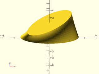
Example 1:
include <BOSL2/std.scad>
skin([octagon(4), circle($fn=70,r=2)], z=[0,3], slices=10);
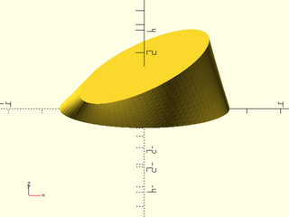
Example 2: Rotating the pentagon place the zero index at different locations, giving a twist
include <BOSL2/std.scad>
skin([rot(90,p=pentagon(4)), circle($fn=80,r=2)], z=[0,3], slices=10);
Example 3: You can untwist it with the "reindex" method
include <BOSL2/std.scad>
skin([rot(90,p=pentagon(4)), circle($fn=80,r=2)], z=[0,3], slices=10, method="reindex");
Example 4: Offsetting the starting edge connects to circles in an interesting way:
include <BOSL2/std.scad>
circ = circle($fn=80, r=3);
skin([circ, rot(110,p=circ)], z=[0,5], slices=20);
Example 5:
include <BOSL2/std.scad>
skin([ yrot(37,p=path3d(circle($fn=128, r=4))), path3d(square(3),3)], method="reindex",slices=10);
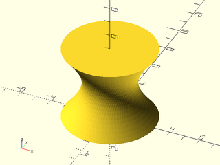
Example 6: Ellipses connected with twist
include <BOSL2/std.scad>
ellipse = xscale(2.5,p=circle($fn=80));
skin([ellipse, rot(45,p=ellipse)], z=[0,1.5], slices=10);
Example 7: Ellipses connected without a twist. (Note ellipses stay in the same position: just the connecting edges are different.)
include <BOSL2/std.scad>
ellipse = xscale(2.5,p=circle($fn=80));
skin([ellipse, rot(45,p=ellipse)], z=[0,1.5], slices=10, method="reindex");
Example 8:
include <BOSL2/std.scad>
$fn=24;
skin([
      yrot(0, p=yscale(2,p=path3d(circle(d=75)))),
      [[40,0,100], [35,-15,100], [20,-30,100],[0,-40,100],[-40,0,100],[0,40,100],[20,30,100], [35,15,100]]
],slices=10);
Example 9:
include <BOSL2/std.scad>
$fn=48;
skin([
    for (b=[0,90]) [
        for (a=[360:-360/$fn:0.01])
            point3d(polar_to_xy((100+50*cos((a+b)*2))/2,a),b/90*100)
    ]
], slices=20);
Example 10: Vaccum connector example from list-comprehension-demos
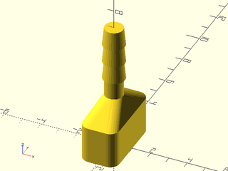
include <BOSL2/std.scad>
include <BOSL2/rounding.scad>
$fn=32;
base = round_corners(square([2,4],center=true), radius=0.5);
skin([
    path3d(base,0),
    path3d(base,2),
    path3d(circle(r=0.5),3),
    path3d(circle(r=0.5),4),
    for(i=[0:2]) each [path3d(circle(r=0.6), i+4),
                       path3d(circle(r=0.5), i+5)]
],slices=0);
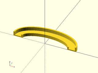
Example 11: Vaccum nozzle example from list-comprehension-demos, using "length" sampling (the default)
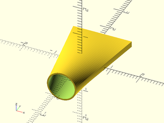
include <BOSL2/std.scad>
xrot(90)down(1.5)
difference() {
    skin(
        [square([2,.2],center=true),
         circle($fn=64,r=0.5)], z=[0,3],
        slices=40,sampling="length",method="reindex");
    skin(
        [square([1.9,.1],center=true),
         circle($fn=64,r=0.45)], z=[-.01,3.01],
        slices=40,sampling="length",method="reindex");
}
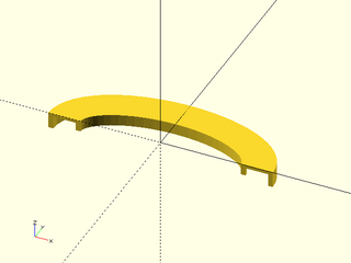
Example 12: Same thing with "segment" sampling
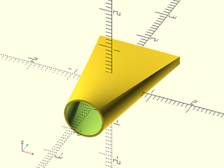
include <BOSL2/std.scad>
xrot(90)down(1.5)
difference() {
    skin(
        [square([2,.2],center=true),
         circle($fn=64,r=0.5)], z=[0,3],
        slices=40,sampling="segment",method="reindex");
    skin(
        [square([1.9,.1],center=true),
         circle($fn=64,r=0.45)], z=[-.01,3.01],
        slices=40,sampling="segment",method="reindex");
}
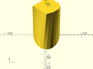
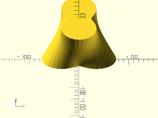
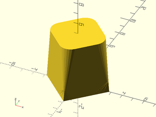
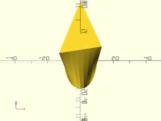
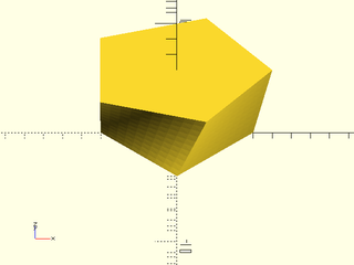
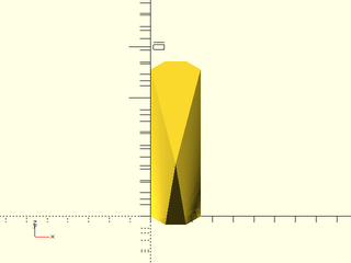
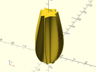
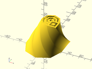
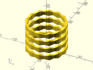
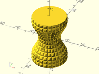
Example 13: Forma Candle Holder (from list-comprehension-demos)
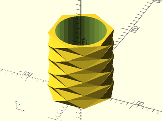
include <BOSL2/std.scad>
r = 50;
height = 140;
layers = 10;
wallthickness = 5;
holeradius = r - wallthickness;
difference() {
    skin([for (i=[0:layers-1]) zrot(-30*i,p=path3d(hexagon(ir=r),i*height/layers))],slices=0);
    up(height/layers) cylinder(r=holeradius, h=height);
}
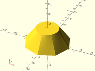
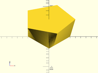
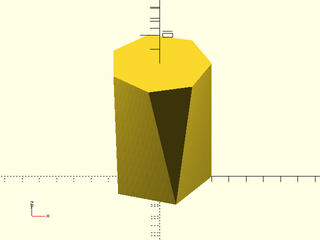
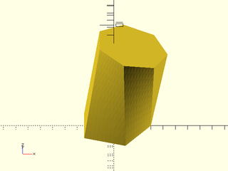
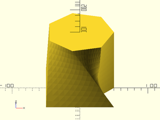
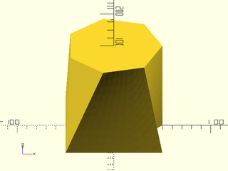
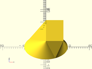
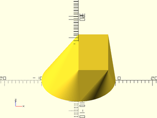
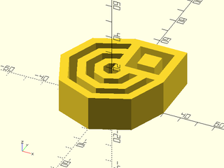
Example 14: A box that is octagonal on the outside and circular on the inside
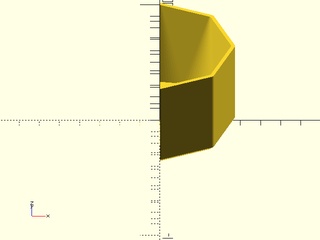
include <BOSL2/std.scad>
height = 45;
sub_base = octagon(d=71, rounding=2, $fn=128);
base = octagon(d=75, rounding=2, $fn=128);
interior = regular_ngon(n=len(base), d=60);
right_half()
  skin([ sub_base, base, base, sub_base, interior], z=[0,2,height, height, 2], slices=0, refine=1, method="reindex");
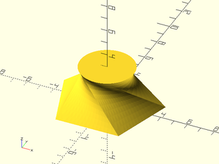
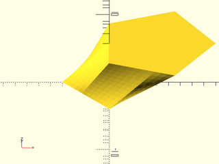
Example 15: Connecting a pentagon and circle with the "tangent" method produces large triangular faces and cone shaped corners.
include <BOSL2/std.scad>
skin([pentagon(4), circle($fn=80,r=2)], z=[0,3], slices=10, method="tangent");
Example 16: rounding corners of a square. Note that $fn makes the number of points constant, and avoiding the rounding=0 case keeps everything simple. In this case, the connections between profiles are linear, so there is no benefit to setting slices bigger than zero.
include <BOSL2/std.scad>
shapes = [for(i=[.01:.045:2])zrot(-i*180/2,cp=[-8,0,0],p=xrot(90,p=path3d(regular_ngon(n=4, side=4, rounding=i, $fn=64))))];
rotate(180) skin( shapes, slices=0);
Example 17: Here's a simplified version of the above, with i=0 included. That first layer doesn't look good.
include <BOSL2/std.scad>
shapes = [for(i=[0:.2:1]) path3d(regular_ngon(n=4, side=4, rounding=i, $fn=32),i*5)];
skin(shapes, slices=0);
Example 18: You can fix it by specifying "tangent" for the first method, but you still need "direct" for the rest.

include <BOSL2/std.scad>
shapes = [for(i=[0:.2:1]) path3d(regular_ngon(n=4, side=4, rounding=i, $fn=32),i*5)];
skin(shapes, slices=0, method=concat(["tangent"],repeat("direct",len(shapes)-2)));
Example 19: Connecting square to pentagon using "direct" method.
include <BOSL2/std.scad>
skin([regular_ngon(n=4, r=4), regular_ngon(n=5,r=5)], z=[0,4], refine=10, slices=10);
Example 20: Connecting square to shifted pentagon using "direct" method.
include <BOSL2/std.scad>
skin([regular_ngon(n=4, r=4), right(4,p=regular_ngon(n=5,r=5))], z=[0,4], refine=10, slices=10);
Example 21: In this example reindexing does not fix the orientation of the triangle because it happens in 3d within skin(), so we have to reverse the triangle manually
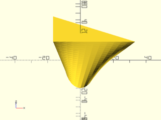
include <BOSL2/std.scad>
ellipse = yscale(3,circle(r=10, $fn=32));
tri = move([-50/3,-9],[[0,0], [50,0], [0,27]]);
skin([ellipse, reverse(tri)], z=[0,20], slices=20, method="reindex");
Example 22: You can get a nicer transition by rotating the polygons for better alignment. You have to resample yourself before calling align_polygon. The orientation is fixed so we do not need to reverse.
include <BOSL2/std.scad>
ellipse = yscale(3,circle(r=10, $fn=32));
tri = move([-50/3,-9],
           subdivide_path([[0,0], [50,0], [0,27]], 32));
aligned = align_polygon(ellipse,tri, [0:5:180]);
skin([ellipse, aligned], z=[0,20], slices=20);
Example 23: The "distance" method is a completely different approach.
include <BOSL2/std.scad>
skin([regular_ngon(n=4, r=4), regular_ngon(n=5,r=5)], z=[0,4], refine=10, slices=10, method="distance");
Example 24: Connecting pentagon to heptagon inserts two triangular faces on each side
include <BOSL2/std.scad>
small = path3d(circle(r=3, $fn=5));
big = up(2,p=yrot( 0,p=path3d(circle(r=3, $fn=7), 6)));
skin([small,big],method="distance", slices=10, refine=10);
Example 25: But just a slight rotation of the top profile moves the two triangles to one end
include <BOSL2/std.scad>
small = path3d(circle(r=3, $fn=5));
big = up(2,p=yrot(14,p=path3d(circle(r=3, $fn=7), 6)));
skin([small,big],method="distance", slices=10, refine=10);
Example 26: Another "distance" example:
include <BOSL2/std.scad>
off = [0,2];
shape = turtle(["right",45,"move", "left",45,"move", "left",45, "move", "jump", [.5+sqrt(2)/2,8]]);
rshape = rot(180,cp=centroid(shape)+off, p=shape);
skin([shape,rshape],z=[0,4], method="distance",slices=10,refine=15);
Example 27: Slightly shifting the profile changes the optimal linkage
include <BOSL2/std.scad>
off = [0,1];
shape = turtle(["right",45,"move", "left",45,"move", "left",45, "move", "jump", [.5+sqrt(2)/2,8]]);
rshape = rot(180,cp=centroid(shape)+off, p=shape);
skin([shape,rshape],z=[0,4], method="distance",slices=10,refine=15);
Example 28: This optimal solution doesn't look terrible:
include <BOSL2/std.scad>
prof1 = path3d([[-50,-50], [-50,50], [50,50], [25,25], [50,0], [25,-25], [50,-50]]);
prof2 = path3d(regular_ngon(n=7, r=50),100);
skin([prof1, prof2], method="distance", slices=10, refine=10);
Example 29: But this one looks better. The "distance" method doesn't find it because it uses two more edges, so it clearly has a higher total edge distance. We force it by doubling the first two vertices of one of the profiles.
include <BOSL2/std.scad>
prof1 = path3d([[-50,-50], [-50,50], [50,50], [25,25], [50,0], [25,-25], [50,-50]]);
prof2 = path3d(regular_ngon(n=7, r=50),100);
skin([repeat_entries(prof1,[2,2,1,1,1,1,1]),
      prof2],
     method="distance", slices=10, refine=10);
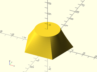
Example 30: The "distance" method will often produces results similar to the "tangent" method if you use it with a polygon and a curve, but the results can also look like this:
include <BOSL2/std.scad>
skin([path3d(circle($fn=128, r=10)), xrot(39, p=path3d(square([8,10]),10))],  method="distance", slices=0);
Example 31: Using the "tangent" method produces:
include <BOSL2/std.scad>
skin([path3d(circle($fn=128, r=10)), xrot(39, p=path3d(square([8,10]),10))],  method="tangent", slices=0);
Example 32: Torus using hexagons and pentagons, where closed=true
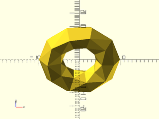
include <BOSL2/std.scad>
hex = right(7,p=path3d(hexagon(r=3)));
pent = right(7,p=path3d(pentagon(r=3)));
N=5;
skin(
     [for(i=[0:2*N-1]) yrot(360*i/2/N, p=(i%2==0 ? hex : pent))],
     refine=1,slices=0,method="distance",closed=true);
Example 33: A smooth morph is achieved when you can calculate all the slices yourself. Since you provide all the slices, set slices=0.
include <BOSL2/std.scad>
skin([for(n=[.1:.02:.5])
         yrot(n*60-.5*60,p=path3d(supershape(step=360/128,m1=5,n1=n, n2=1.7),5-10*n))],
     slices=0);
Example 34: Another smooth supershape morph:
include <BOSL2/std.scad>
skin([for(alpha=[-.2:.05:1.5])
         path3d(supershape(step=360/256,m1=7, n1=lerp(2,3,alpha),
                           n2=lerp(8,4,alpha), n3=lerp(4,17,alpha)),alpha*5)],
     slices=0);
Example 35: Several polygons connected using "distance"
include <BOSL2/std.scad>
skin([regular_ngon(n=4, r=3),
      regular_ngon(n=6, r=3),
      regular_ngon(n=9, r=4),
      rot(17,p=regular_ngon(n=6, r=3)),
      rot(37,p=regular_ngon(n=4, r=3))],
     z=[0,2,4,6,9], method="distance", slices=10, refine=10);
Example 36: Vertex count of the polygon changes at every profile
include <BOSL2/std.scad>
skin([
    for (ang = [0:10:90])
    rot([0,ang,0], cp=[200,0,0], p=path3d(circle(d=100,$fn=12-(ang/10))))
],method="distance",slices=10,refine=10);
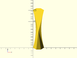
Example 37: Möbius Strip. This is a tricky model because when you work your way around to the connection, the direction of the profiles is flipped, so how can the proper geometry be created? The trick is to duplicate the first profile and turn the caps off. The model closes up and forms a valid polyhedron.

include <BOSL2/std.scad>
skin([
  for (ang = [0:5:360])
  rot([0,ang,0], cp=[100,0,0], p=rot(ang/2, p=path3d(square([1,30],center=true))))
], caps=false, slices=0, refine=20);
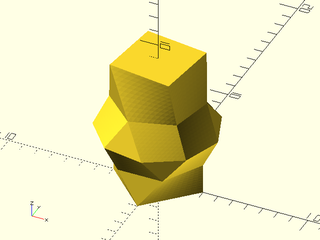
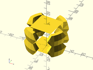
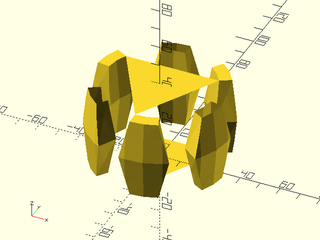
Example 38: This model of two scutoids packed together is based on https://www.thingiverse.com/thing:3024272 by mathgrrl
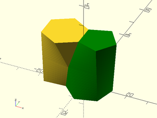
include <BOSL2/std.scad>
sidelen = 10;  // Side length of scutoid
height = 25;   // Height of scutoid
angle = -15;   // Angle (twists the entire form)
push = -5;     // Push (translates the base away from the top)
flare = 1;     // Flare (the two pieces will be different unless this is 1)
midpoint = .5; // Height of the extra vertex (as a fraction of total height); the two pieces will be different unless this is .5)
pushvec = rot(angle/2,p=push*RIGHT);  // Push direction is the average of the top and bottom mating edges
pent = path3d(apply(move(pushvec)*rot(angle),pentagon(side=sidelen,align_side=RIGHT,anchor="side0")));
hex = path3d(hexagon(side=flare*sidelen, align_side=RIGHT, anchor="side0"),height);
pentmate = path3d(pentagon(side=flare*sidelen,align_side=LEFT,anchor="side0"),height);
          // Native index would require mapping first and last vertices together, which is not allowed, so shift
hexmate = list_rotate(
                        path3d(apply(move(pushvec)*rot(angle),hexagon(side=sidelen,align_side=LEFT,anchor="side0"))),
                        -1);
join_vertex = lerp(
                    mean(select(hex,1,2)),     // midpoint of "extra" hex edge
                    mean(select(hexmate,0,1)), // midpoint of "extra" hexmate edge
                    midpoint);
augpent = repeat_entries(pent, [1,2,1,1,1]);         // Vertex 1 will split at the top forming a triangular face with the hexagon
augpent_mate = repeat_entries(pentmate,[2,1,1,1,1]); // For mating pentagon it is vertex 0 that splits
           // Middle is the interpolation between top and bottom except for the join vertex, which is doubled because it splits
middle = list_set(lerp(augpent,hex,midpoint),[1,2],[join_vertex,join_vertex]);
middle_mate = list_set(lerp(hexmate,augpent_mate,midpoint), [0,1], [join_vertex,join_vertex]);
skin([augpent,middle,hex],  slices=10, refine=10, sampling="segment");
color("green")skin([augpent_mate,middle_mate,hexmate],  slices=10,refine=10, sampling="segment");
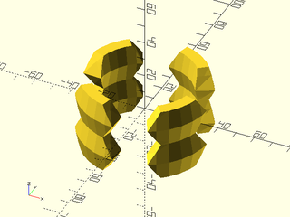
Example 39: If you create a self-intersecting polyhedron the result is invalid. In some cases self-intersection may be obvous. Here is a more subtle example.
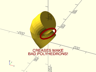
include <BOSL2/std.scad>
skin([
       for (a = [0:30:180]) let(
           pos  = [-60*sin(a),     0, a    ],
           pos2 = [-60*sin(a+0.1), 0, a+0.1]
       ) move(pos,
           p=rot(from=UP, to=pos2-pos,
               p=path3d(circle(d=150))
           )
       )
   ],refine=1,slices=0);
   color("red") {
       zrot(25) fwd(130) xrot(75) {
           linear_extrude(height=0.1) {
               ydistribute(25) {
                   text(text="BAD POLYHEDRONS!", size=20, halign="center", valign="center");
                   text(text="CREASES MAKE", size=20, halign="center", valign="center");
               }
           }
       }
       up(160) zrot(25) fwd(130) xrot(75) {
           stroke(zrot(30, p=yscale(0.5, p=circle(d=120))),width=10,closed=true);
       }
   }
Synopsis: Create a linear extrusion from a path, with optional texturing. [VNF] [Geom]
Topics: Extrusion, Textures, Sweep
See Also: rotate_sweep(), sweep(), spiral_sweep(), path_sweep(), offset_sweep()
Usage: As Module
- linear_sweep(region, [height], [center=], [slices=], [twist=], [scale=], [style=], [caps=], [convexity=]) [ATTACHMENTS];
Usage: With Texturing
- linear_sweep(region, [height], [center=], texture=, [tex_size=]|[tex_reps=], [tex_depth=], [style=], [tex_samples=], ...) [ATTACHMENTS];
Usage: As Function
- vnf = linear_sweep(region, [height], [center=], [slices=], [twist=], [scale=], [style=], [caps=]);
- vnf = linear_sweep(region, [height], [center=], texture=, [tex_size=]|[tex_reps=], [tex_depth=], [style=], [tex_samples=], ...);
Description:
If called as a module, creates a polyhedron that is the linear extrusion of the given 2D region or polygon.
If called as a function, returns a VNF that can be used to generate a polyhedron of the linear extrusion
of the given 2D region or polygon. The benefit of using this, over using linear_extrude region(rgn) is
that it supports anchor, spin, orient and attachments. You can also make more refined
twisted extrusions by using maxseg to subsample flat faces.
Anchoring for linear_sweep is based on the anchors for the swept region rather than from the polyhedron that is created. This can produce more
predictable anchors for LEFT, RIGHT, FWD and BACK in many cases, but the anchors may only
be aproximately correct for twisted objects, and corner anchors may point in unexpected directions in some cases.
If you need anchors directly computed from the surface you can pass the vnf from linear_sweep
to vnf_polyhedron(), which will compute anchors directly from the full VNF.
Arguments:
| By Position | What it does |
|---|---|
region |
The 2D Region or polygon that is to be extruded. |
h / height / l / length
|
The height to extrude the region. Default: 1 |
center |
If true, the created polyhedron will be vertically centered. If false, it will be extruded upwards from the XY plane. Default: false
|
| By Name | What it does |
|---|---|
twist |
The number of degrees to rotate the top of the shape, clockwise around the Z axis, relative to the bottom. Default: 0 |
scale |
The amount to scale the top of the shape, in the X and Y directions, relative to the size of the bottom. Default: 1 |
shift |
The amount to shift the top of the shape, in the X and Y directions, relative to the position of the bottom. Default: [0,0] |
slices |
The number of slices to divide the shape into along the Z axis, to allow refinement of detail, especially when working with a twist. Default: twist/5
|
maxseg |
If given, then any long segments of the region will be subdivided to be shorter than this length. This can refine twisting flat faces a lot. Default: undef (no subsampling) |
texture |
A texture name string, or a rectangular array of scalar height values (0.0 to 1.0), or a VNF tile that defines the texture to apply to vertical surfaces. See texture() for what named textures are supported. |
tex_size |
An optional 2D target size for the textures. Actual texture sizes will be scaled somewhat to evenly fit the available surface. Default: [5,5]
|
tex_reps |
If given instead of tex_size, a 2-vector giving the number of texture tile repetitions in the horizontal and vertical directions on the extrusion. |
tex_inset |
If numeric, lowers the texture into the surface by the specified proportion, e.g. 0.5 would lower it half way into the surface. If true, insets by exactly its full depth. Default: false
|
tex_rot |
Rotate texture by specified angle, which must be a multiple of 90 degrees. Default: 0 |
tex_depth |
Specify texture depth; if negative, invert the texture. Default: 1. |
tex_samples |
Minimum number of "bend points" to have in VNF texture tiles. Default: 8 |
style |
The style to use when triangulating the surface of the object. Valid values are "default", "alt", or "quincunx". |
caps |
If false do not create end caps. Can be a boolean vector. Default: true |
convexity |
Max number of surfaces any single ray could pass through. Module use only. |
cp |
Centerpoint for determining intersection anchors or centering the shape. Determines the base of the anchor vector. Can be "centroid", "mean", "box" or a 3D point. Default: "centroid"
|
atype |
Set to "hull" or "intersect" to select anchor type. Default: "hull" |
anchor |
Translate so anchor point is at origin (0,0,0). See anchor. Default: "origin"
|
spin |
Rotate this many degrees around the Z axis after anchor. See spin. Default: 0
|
orient |
Vector to rotate top towards, after spin. See orient. Default: UP
|
Anchor Types:
| Anchor Type | What it is |
|---|---|
| "hull" | Anchors to the virtual convex hull of the shape. |
| "intersect" | Anchors to the surface of the shape. |
| "bbox" | Anchors to the bounding box of the extruded shape. |
Extra Anchors:
| Anchor Name | Position |
|---|---|
| "origin" | Centers the extruded shape vertically only, but keeps the original path positions in the X and Y. Oriented UP. |
| "original_base" | Keeps the original path positions in the X and Y, but at the bottom of the extrusion. Oriented UP. |
Example 1: Extruding a Compound Region.
include <BOSL2/std.scad>
rgn1 = [for (d=[10:10:60]) circle(d=d,$fn=8)];
rgn2 = [square(30,center=false)];
rgn3 = [for (size=[10:10:20]) move([15,15],p=square(size=size, center=true))];
mrgn = union(rgn1,rgn2);
orgn = difference(mrgn,rgn3);
linear_sweep(orgn,height=20,convexity=16);
Example 2: With Twist, Scale, Shift, Slices and Maxseg.
include <BOSL2/std.scad>
rgn1 = [for (d=[10:10:60]) circle(d=d,$fn=8)];
rgn2 = [square(30,center=false)];
rgn3 = [
    for (size=[10:10:20])
    apply(
       move([15,15]),
       square(size=size, center=true)
    )
];
mrgn = union(rgn1,rgn2);
orgn = difference(mrgn,rgn3);
linear_sweep(
    orgn, height=50, maxseg=2, slices=40,
    twist=90, scale=0.5, shift=[10,5],
    convexity=16
);
Example 3: Anchors on an Extruded Region
include <BOSL2/std.scad>
rgn1 = [for (d=[10:10:60]) circle(d=d,$fn=8)];
rgn2 = [square(30,center=false)];
rgn3 = [
    for (size=[10:10:20])
    apply(
        move([15,15]),
        rect(size=size)
    )
];
mrgn = union(rgn1,rgn2);
orgn = difference(mrgn,rgn3);
linear_sweep(orgn,height=20,convexity=16)
    show_anchors();
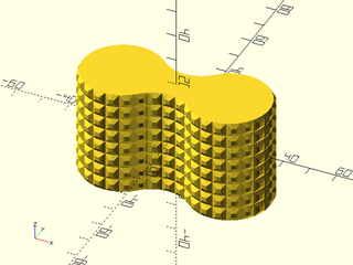
Example 4: "diamonds" texture.
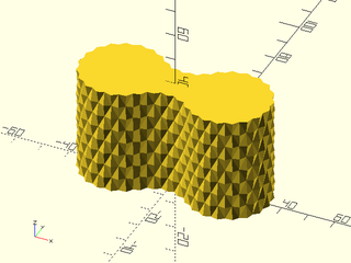
include <BOSL2/std.scad>
path = glued_circles(r=15, spread=40, tangent=45);
linear_sweep(
    path, texture="diamonds", tex_size=[5,10],
    h=40, style="concave");
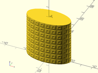
Example 5: "pyramids" texture.
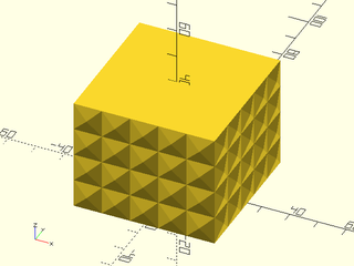
include <BOSL2/std.scad>
linear_sweep(
    rect(50), texture="pyramids", tex_size=[10,10],
    h=40, style="convex");
Example 6: "bricks_vnf" texture.
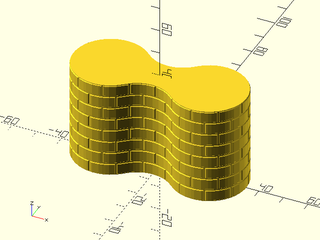
include <BOSL2/std.scad>
path = glued_circles(r=15, spread=40, tangent=45);
linear_sweep(
    path, texture="bricks_vnf", tex_size=[10,10],
    tex_depth=0.25, h=40);
Example 7: User defined heightfield texture.
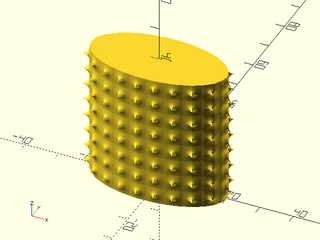
include <BOSL2/std.scad>
path = ellipse(r=[20,10]);
texture = [for (i=[0:9])
    [for (j=[0:9])
        1/max(0.5,norm([i,j]-[5,5])) ]];
linear_sweep(
    path, texture=texture, tex_size=[5,5],
    h=40, style="min_edge", anchor=BOT);
Example 8: User defined VNF tile texture.
include <BOSL2/std.scad>
path = ellipse(r=[20,10]);
tex = let(n=16,m=0.25) [
     [
         each resample_path(path3d(square(1)),n),
         each move([0.5,0.5],
             p=path3d(circle(d=0.5,$fn=n),m)),
         [1/2,1/2,0],
     ], [
         for (i=[0:1:n-1]) each [
             [i,(i+1)%n,(i+3)%n+n],
             [i,(i+3)%n+n,(i+2)%n+n],
             [2*n,n+i,n+(i+1)%n],
         ]
     ]
];
linear_sweep(path, texture=tex, tex_size=[5,5], h=40);
Example 9: Textured with twist and scale.
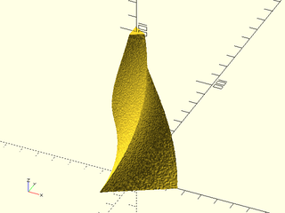
include <BOSL2/std.scad>
linear_sweep(regular_ngon(n=3, d=50),
    texture="rough", h=100, tex_depth=2,
    tex_size=[20,20], style="min_edge",
    convexity=10, scale=0.2, twist=120);
Example 10: As Function
include <BOSL2/std.scad>
path = glued_circles(r=15, spread=40, tangent=45);
vnf = linear_sweep(
    path, h=40, texture="trunc_pyramids", tex_size=[5,5],
    tex_depth=1, style="convex");
vnf_polyhedron(vnf, convexity=10);
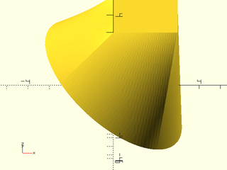
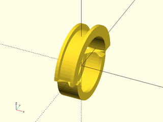
Example 11: VNF tile that has no top/bottom edges and produces a disconnected result
include <BOSL2/std.scad>
shape = skin([rect(2/5),
              rect(2/3),
              rect(2/5)],
             z=[0,1/2,1],
             slices=0,
             caps=false);
tile = move([0,1/2,2/3],yrot(90,shape));
linear_sweep(circle(20), texture=tile,
             tex_size=[10,10],tex_depth=5,
             h=40,convexity=4);
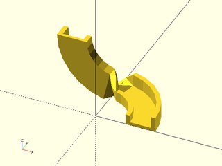
Example 12: The same tile from above, turned 90 degrees, creates problems at the ends, because the end cap is not a connected polygon. When the ends are disconnected you may find that some parts of the end cap are missing and spurious polygons included.
include <BOSL2/std.scad>
shape = skin([rect(2/5),
              rect(2/3),
              rect(2/5)],
             z=[0,1/2,1],
             slices=0,
             caps=false);
tile = move([1/2,1,2/3],xrot(90,shape));
linear_sweep(circle(20), texture=tile,
             tex_size=[30,20],tex_depth=15,
             h=40,convexity=4);
Example 13: This example shows some endcap polygons missing and a spurious triangle
include <BOSL2/std.scad>
shape = skin([rect(2/5),
              rect(2/3),
              rect(2/5)],
             z=[0,1/2,1],
             slices=0,
             caps=false);
tile = xscale(.5,move([1/2,1,2/3],xrot(90,shape)));
doubletile = vnf_join([tile, right(.5,tile)]);
linear_sweep(circle(20), texture=doubletile,
             tex_size=[45,45],tex_depth=15, h=40);
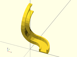
Example 14: You can fix ends for disconnected cases using top_half() and bottom_half()
include <BOSL2/std.scad>
shape = skin([rect(2/5),
              rect(2/3),
              rect(2/5)],
             z=[0,1/2,1],
             slices=0,
             caps=false);
tile = move([1/2,1,2/3],xrot(90,shape));
vnf_polyhedron(
  top_half(
    bottom_half(
      linear_sweep(circle(20), texture=tile,
                  tex_size=[30,20],tex_depth=15,
                  h=40.2,caps=false),
    z=20),
  z=-20));
Synopsis: Create a surface of revolution from a path with optional texturing. [VNF] [Geom]
Topics: Extrusion, Sweep, Revolution, Textures
See Also: linear_sweep(), sweep(), spiral_sweep(), path_sweep(), offset_sweep()
Usage: As Function
- vnf = rotate_sweep(shape, [angle], ...);
Usage: As Module
- rotate_sweep(shape, [angle], ...) [ATTACHMENTS];
Usage: With Texturing
- rotate_sweep(shape, texture=, [tex_size=]|[tex_reps=], [tex_depth=], [tex_samples=], [tex_rot=], [tex_inset=], ...) [ATTACHMENTS];
Description:
Takes a polygon or region and sweeps it in a rotation around the Z axis, with optional texturing. When called as a function, returns a VNF. When called as a module, creates the sweep as geometry.
Arguments:
| By Position | What it does |
|---|---|
shape |
The polygon or region to sweep around the Z axis. |
angle |
If given, specifies the number of degrees to sweep the shape around the Z axis, counterclockwise from the X+ axis. Default: 360 (full rotation) |
| By Name | What it does |
|---|---|
texture |
A texture name string, or a rectangular array of scalar height values (0.0 to 1.0), or a VNF tile that defines the texture to apply to vertical surfaces. See texture() for what named textures are supported. |
tex_size |
An optional 2D target size for the textures. Actual texture sizes will be scaled somewhat to evenly fit the available surface. Default: [5,5]
|
tex_reps |
If given instead of tex_size, a 2-vector giving the number of texture tile repetitions in the direction perpendicular to extrusion and in the direction parallel to extrusion. |
tex_inset |
If numeric, lowers the texture into the surface by the specified proportion, e.g. 0.5 would lower it half way into the surface. If true, insets by exactly its full depth. Default: false
|
tex_rot |
Rotate texture by specified angle, which must be a multiple of 90 degrees. Default: 0 |
tex_depth |
Specify texture depth; if negative, invert the texture. Default: 1. |
tex_samples |
Minimum number of "bend points" to have in VNF texture tiles. Default: 8 |
style |
vnf_vertex_array() style. Default: "min_edge" |
closed |
If false, and shape is given as a path, then the revolved path will be sealed to the axis of rotation with untextured caps. Default: true
|
convexity |
(Module only) Convexity setting for use with polyhedron. Default: 10 |
cp |
Centerpoint for determining "intersect" anchors or centering the shape. Determintes the base of the anchor vector. Can be "centroid", "mean", "box" or a 3D point. Default: "centroid" |
atype |
Select "hull" or "intersect" anchor types. Default: "hull" |
anchor |
Translate so anchor point is at the origin. Default: "origin" |
spin |
Rotate this many degrees around Z axis after anchor. Default: 0 |
orient |
Vector to rotate top towards after spin (module only) |
Anchor Types:
| Anchor Type | What it is |
|---|---|
| "hull" | Anchors to the virtual convex hull of the shape. |
| "intersect" | Anchors to the surface of the shape. |
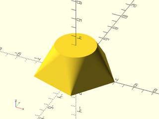
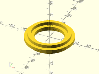
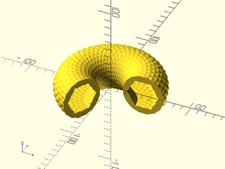
Example 1:
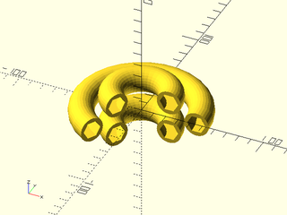
include <BOSL2/std.scad>
rgn = [
    for (a = [0, 120, 240]) let(
        cp = polar_to_xy(15, a) + [30,0]
    ) each [
        move(cp, p=circle(r=10)),
        move(cp, p=hexagon(d=15)),
    ]
];
rotate_sweep(rgn, angle=240);
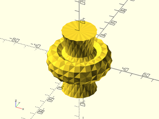
Example 2:
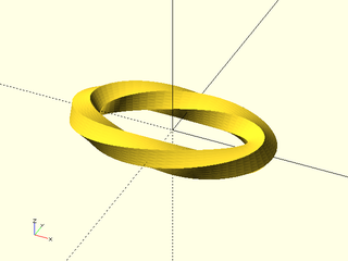
include <BOSL2/std.scad>
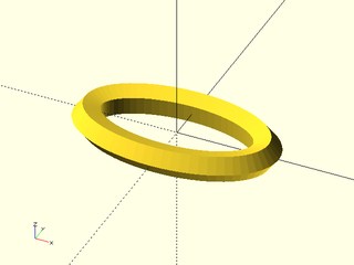
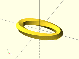
rgn = right(30, p=union([for (a = [0, 90]) rot(a, p=rect([15,5]))]));
rotate_sweep(rgn);
Example 3:
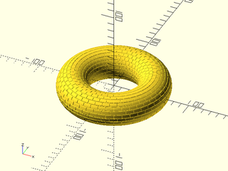
include <BOSL2/std.scad>
path = right(50, p=circle(d=40));
rotate_sweep(path, texture="bricks_vnf", tex_size=[10,10], tex_depth=0.5, style="concave");
Example 4:
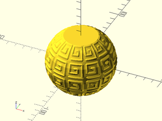
include <BOSL2/std.scad>
tex = [
[0, 0, 0, 0, 0, 0, 0, 0, 0, 0, 0],
[0, 0, 1, 1, 1, 1, 1, 1, 1, 1, 1],
[0, 0, 1, 0, 0, 0, 0, 0, 0, 0, 1],
[0, 0, 1, 0, 0, 0, 0, 0, 0, 0, 1],
[0, 0, 1, 0, 0, 1, 1, 1, 0, 0, 1],
[0, 0, 1, 0, 0, 0, 0, 1, 0, 0, 1],
[0, 0, 1, 0, 0, 0, 0, 1, 0, 0, 1],
[0, 0, 1, 1, 1, 1, 1, 1, 0, 0, 1],
[0, 0, 0, 0, 0, 0, 0, 0, 0, 0, 1],
[0, 0, 0, 0, 0, 0, 0, 0, 0, 0, 1],
[0, 0, 1, 1, 1, 1, 1, 1, 1, 1, 1],
[0, 0, 0, 0, 0, 0, 0, 0, 0, 0, 0],
];
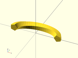
path = arc(cp=[0,0], r=40, start=60, angle=-120);
rotate_sweep(
path, closed=false,
texture=tex, tex_size=[20,20],
tex_depth=1, style="concave");
Example 5:
include <BOSL2/std.scad>
include <BOSL2/beziers.scad>
bezpath = [
    [15, 30], [10,15],
    [10,  0], [20, 10], [30,12],
    [30,-12], [20,-10], [10, 0],
    [10,-15], [15,-30]
];
path = bezpath_curve(bezpath, splinesteps=32);
rotate_sweep(
    path, closed=false,
    texture="diamonds", tex_size=[10,10],
    tex_depth=1, style="concave");
Example 6:
include <BOSL2/std.scad>
path = [
    [20, 30], [20, 20],
    each arc(r=20, corner=[[20,20],[10,0],[20,-20]]),
    [20,-20], [20,-30],
];
vnf = rotate_sweep(
    path, closed=false,
    texture="trunc_pyramids",
    tex_size=[5,5], tex_depth=1,
    style="convex");
vnf_polyhedron(vnf, convexity=10);
Example 7:
include <BOSL2/std.scad>
rgn = [
    right(40, p=circle(d=50)),
    right(40, p=circle(d=40,$fn=6)),
];
rotate_sweep(
    rgn, texture="diamonds",
    tex_size=[10,10], tex_depth=1,
    angle=240, style="concave");
Synopsis: Sweep a path along a helix. [VNF] [Geom]
Topics: Extrusion, Sweep, Spiral
See Also: thread_helix(), linear_sweep(), rotate_sweep(), sweep(), path_sweep(), offset_sweep()
Usage: As Module
- spiral_sweep(poly, h, r|d=, turns, [taper=], [center=], [taper1=], [taper2=], [internal=], ...)[ATTACHMENTS];
- spiral_sweep(poly, h, r1=|d1=, r2=|d2=, turns, [taper=], [center=], [taper1=], [taper2=], [internal=], ...)[ATTACHMENTS];
Usage: As Function
- vnf = spiral_sweep(poly, h, r|d=, turns, ...);
- vnf = spiral_sweep(poly, h, r1=|d1=, r1=|d2=, turns, ...);
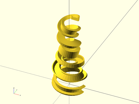
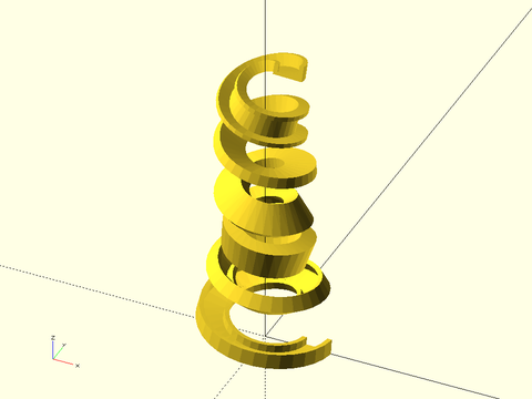
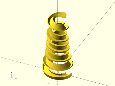
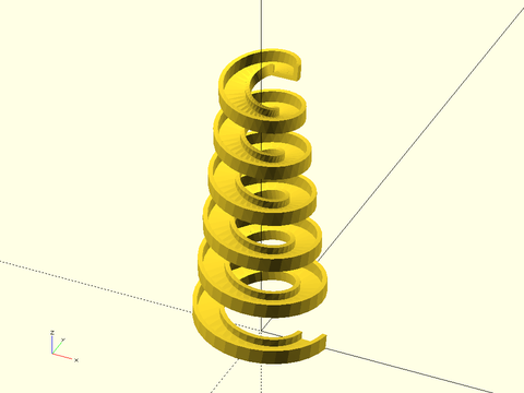
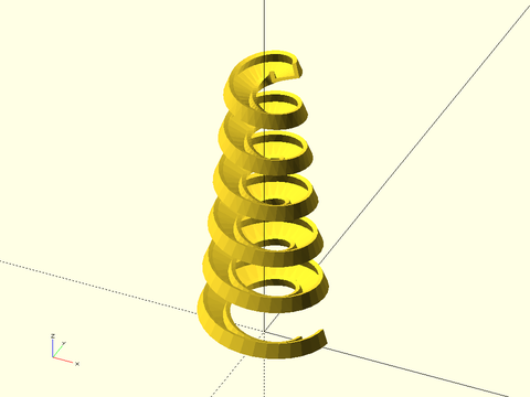
Description:
Takes a closed 2D polygon path, centered on the XY plane, and sweeps/extrudes it along a 3D spiral path of a given radius, height and degrees of rotation. The origin in the profile traces out the helix of the specified radius. If turns is positive the path will be right-handed; if turns is negative the path will be left-handed. Such an extrusion can be used to make screw threads.
The lead_in options specify a lead-in section where the ends of the spiral scale down to avoid a sharp cut face at the ends.
You can specify the length of this scaling directly with the lead_in parameters or as an angle using the lead_in_ang parameters.
If you give a positive value, the extrusion is lengthenend by the specified distance or angle; if you give a negative
value then the scaled end is included in the extrusion length specified by turns. If the value is zero then no scaled ends
are produced. The shape of the scaled ends can be controlled with the lead_in_shape parameter. Supported options are "sqrt", "linear"
"smooth" and "cut".
The inside argument changes how the extrusion lead-in sections are formed. If it is true then they scale towards the outside, like would be needed for internal threading. If internal is fale then the lead-in sections scale towards the inside, like would be appropriate for external threads.
Arguments:
| By Position | What it does |
|---|---|
poly |
Array of points of a polygon path, to be extruded. |
h |
height of the spiral extrusion path |
r |
Radius of the spiral extrusion path |
turns |
number of revolutions to include in the spiral |
| By Name | What it does |
|---|---|
d |
Diameter of the spiral extrusion path. |
d1 / r1
|
Bottom inside diameter or radius of spiral to extrude along. |
d2 / r2
|
Top inside diameter or radius of spiral to extrude along. |
lead_in |
Specify linear length of the lead-in scaled section of the spiral. Default: 0 |
lead_in1 |
Specify linear length of the lead-in scaled section of the spiral at the bottom |
lead_in2 |
Specify linear length of the lead-in scaled section of the spiral at the top |
lead_in_ang |
Specify angular length of the lead-in scaled section of the spiral |
lead_in_ang1 |
Specify angular length of the lead-in scaled section of the spiral at the bottom |
lead_in_ang2 |
Specify angular length of the lead-in scaled section of the spiral at the top |
lead_in_shape |
Specify the shape of the thread lead in by giving a text string or function. Default: "sqrt" |
lead_in_shape1 |
Specify the shape of the thread lead-in at the bottom by giving a text string or function. |
lead_in_shape2 |
Specify the shape of the thread lead-in at the top by giving a text string or function. |
lead_in_sample |
Factor to increase sample rate in the lead-in section. Default: 10 |
internal |
if true make internal threads. The only effect this has is to change how the extrusion lead-in section are formed. When true, the extrusion scales towards the outside; when false, it scales towards the inside. Default: false |
anchor |
Translate so anchor point is at origin (0,0,0). See anchor. Default: CENTER
|
spin |
Rotate this many degrees around the Z axis after anchor. See spin. Default: 0
|
orient |
Vector to rotate top towards, after spin. See orient. Default: UP
|
Example 1:
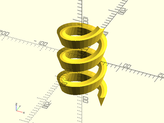
include <BOSL2/std.scad>
poly = [[-10,0], [-3,-5], [3,-5], [10,0], [0,-30]];
spiral_sweep(poly, h=200, r=50, turns=3, $fn=36);
Synopsis: Sweep a 2d polygon path along a 2d or 3d path. [VNF] [Geom]
Topics: Extrusion, Sweep, Paths
See Also: linear_sweep(), rotate_sweep(), sweep(), spiral_sweep(), path_sweep2d(), offset_sweep()
Usage: As module
- path_sweep(shape, path, [method], [normal=], [closed=], [twist=], [twist_by_length=], [symmetry=], [scale=], [scale_by_length=], [last_normal=], [tangent=], [uniform=], [relaxed=], [caps=], [style=], [convexity=], [anchor=], [cp=], [spin=], [orient=], [atype=]) [ATTACHMENTS];
Usage: As function
- vnf = path_sweep(shape, path, [method], [normal=], [closed=], [twist=], [twist_by_length=], [symmetry=], [scale=], [scale_by_length=], [last_normal=], [tangent=], [uniform=], [relaxed=], [caps=], [style=], [transforms=], [anchor=], [cp=], [spin=], [orient=], [atype=]);
Description:
Takes as input shape, a 2D polygon path (list of points), and path, a 2d or 3d path (also a list of points)
and constructs a polyhedron by sweeping the shape along the path. When run as a module returns the polyhedron geometry.
When run as a function returns a VNF by default or if you set transforms=true then it returns a list of transformations suitable as input to sweep.
The sweeping process places one copy of the shape for each point in the path. The origin in shape is translated to
the point in path. The normal vector of the shape, which points in the Z direction, is aligned with the tangent
vector for the path, so this process is constructing a shape whose normal cross sections are equal to your specified shape.
If you do not supply a list of tangent vectors then an approximate tangent vector is computed
based on the path points you supply using path_tangents().
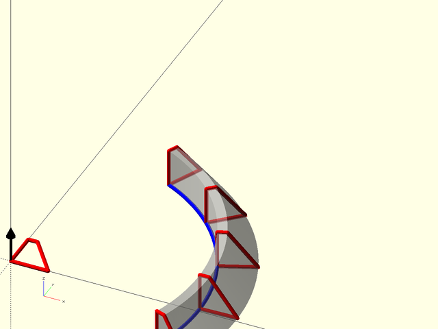
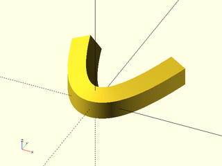
Figure 1: This example shows how the shape, in this case the quadrilateral defined by [[0, 0], [0, 1], [0.25, 1], [1, 0]], appears as the cross section of the swept polyhedron. The blue line shows the path. The normal vector to the shape is shown in black; it is based at the origin and points upwards in the Z direction. The sweep aligns this normal vector with the blue path tangent, which in this case, flips the shape around. Note that for a 2D path like this one, the Y direction in the shape is mapped to the Z direction in the sweep.
In the figure you can see that the swept polyhedron, shown in transparent gray, has the quadrilateral as its cross section. The quadrilateral is positioned perpendicular to the path, which is shown in blue, so that the normal vector for the quadrilateral is parallel to the tangent vector for the path. The origin for the shape is the point which follows the path. For a 2D path, the Y axis of the shape is mapped to the Z axis and in this case, pointing the quadrilateral's normal vector (in black) along the tangent line of the path, which is going in the direction of the blue arrow, requires that the quadrilateral be "turned around". If we reverse the order of points in the path we get a different result:
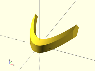
Figure 2: The same sweep operation with the path traveling in the opposite direction. Note that in order to line up the normal correctly, the shape is reversed compared to Figure 1, so the resulting sweep looks quite different.
If your shape is too large for the curves in the path you can create a situation where the shapes cross each
other. This results in an invalid polyhedron, which may appear OK when previewed or rendered alone, but will give rise
to cryptic CGAL errors when rendered with a second object in your model. You may be able to use path_sweep2d()
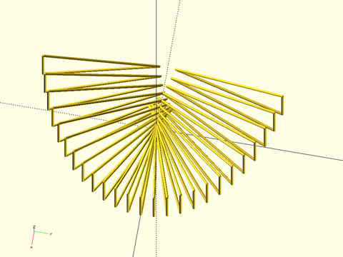
to produce a valid model in cases like this. You can debug models like this using the profiles=true option which will show all
the cross sections in your polyhedron. If any of them intersect, the polyhedron will be invalid.
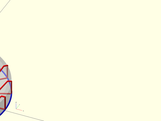
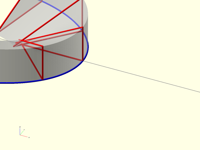
Figure 3: We have scaled the path to an ellipse and show a large triangle as the shape. The triangle is sometimes bigger than the local radius of the path, leading to an invalid polyhedron, which you can identify because the red lines cross in the middle.
During the sweep operation the shape's normal vector aligns with the tangent vector of the path. Note that
this leaves an ambiguity about how the shape is rotated as it sweeps along the path.
For 2D paths, this ambiguity is resolved by aligning the Y axis of the shape to the Z axis of the swept polyhedron.
You can force the shape to twist as it sweeps along the path using the twist parameter, which specifies the total
number of degrees to twist along the whole swept polyhedron. This produces a result like the one shown below.
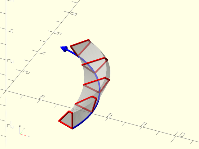
Figure 4: The shape twists as we sweep. Note that it still aligns the origin in the shape with the path, and still aligns the normal vector with the path tangent vector.
The twist argument adds the specified number of degrees of twist into the model, and it may be positive or
negative. When closed=true the starting shape and ending shape must match to avoid a sudden extreme twist at the
joint. By default twist is therefore required to be a multiple of 360. However, if your shape has rotational
symmetry, this requirement is overly strict. You can specify the symmetry using the symmetry argument, and then
you can choose smaller twists consistent with the specified symmetry. The symmetry argument gives the number of
rotations that map the shape exactly onto itself, so a pentagon has 5-fold symmetry. This argument is only valid
for closed sweeps. When you specify symmetry, the twist must be a multiple of 360/symmetry.
The twist is normally spread uniformly along your shape based on the path length. If you set twist_by_length to
false then the twist will be uniform based on the point count of your path. Twisted shapes will produce twisted
faces, so if you want them to look good you should use lots of points on your path and also lots of points on the
shape. If your shape is a simple polygon, use subdivide_path() to increase
the number of points.
As noted above, the sweep process has an ambiguity regarding the twist. For 2D paths it is easy to resolve this
ambiguity by aligning the Y axis in the shape to the Z axis in the swept polyhedron. When the path is
three-dimensional, things become more complex. It is no longer possible to use a simple alignment rule like the
one we use in 2D. You may find that the shape rotates unexpectedly around its axis as it traverses the path. The
method parameter allows you to specify how the shapes are aligned, resulting in different twist in the resulting
polyhedron. You can choose from three different methods for selecting the rotation of your shape. None of these
methods will produce good, or even valid, results on all inputs, so it is important to select a suitable method.
The three methods you can choose using the method parameter are:
The "incremental" method (the default) works by adjusting the shape at each step by the minimal rotation that makes the shape normal to the tangent
at the next point. This method is robust in that it always produces a valid result for well-behaved paths with sufficiently high
sampling. Unfortunately, it can produce a large amount of undesirable twist. When constructing a closed shape this algorithm in
its basic form provides no guarantee that the start and end shapes match up. To prevent a sudden twist at the last segment,
the method calculates the required twist for a good match and distributes it over the whole model (as if you had specified a
twist amount). If you specify symmetry this may allow the algorithm to choose a smaller twist for this alignment.
To start the algorithm, we need an initial condition. This is supplied by
using the normal argument to give a direction to align the Y axis of your shape. By default the normal points UP if the path
makes an angle of 45 deg or less with the xy plane and it points BACK if the path makes a higher angle with the XY plane. You
can also supply last_normal which provides an ending orientation constraint. Be aware that the curve may still exhibit
twisting in the middle. This method is the default because it is the most robust, not because it generally produces the best result.
The "natural" method works by computing the Frenet frame at each point on the path. This is defined by the tangent to the curve and the normal which lies in the plane defined by the curve at each point. This normal points in the direction of curvature of the curve. The result is a very well behaved set of shape positions without any unexpected twisting—as long as the curvature never falls to zero. At a point of zero curvature (a flat point), the curve does not define a plane and the natural normal is not defined. Furthermore, even if you skip over this troublesome point so the normal is defined, it can change direction abruptly when the curvature is zero, leading to a nasty twist and an invalid model. A simple example is a circular arc joined to another arc that curves the other direction. Note that the X axis of the shape is aligned with the normal from the Frenet frame.
The "manual" method allows you to specify your desired normal either globally with a single vector, or locally with
a list of normal vectors for every path point. The normal you supply is projected to be orthogonal to the tangent to the
path and the Y direction of your shape will be aligned with the projected normal. (Note this is different from the "natural" method.)
Careless choice of a normal may result in a twist in the shape, or an error if your normal is parallel to the path tangent.
If you set relax=true then the condition that the cross sections are orthogonal to the path is relaxed and the swept object
uses the actual specified normal. In this case, the tangent is projected to be orthogonal to your supplied normal to define
the cross section orientation. Specifying a list of normal vectors gives you complete control over the orientation of your
cross sections and can be useful if you want to position your model to be on the surface of some solid.
You can also apply scaling to the profile along the path. You can give a list of scalar scale factors or a list of 2-vector scale. In the latter scale the x and y scales of the profile are scaled separately before the profile is placed onto the path. For non-closed paths you can also give a single scale value or a 2-vector which is treated as the final scale. The intermediate sections are then scaled by linear interpolation either relative to length (if scale_by_length is true) or by point count otherwise.
You can use set transforms to true to return a list of transformation matrices instead of the swept shape. In this case, you can
often omit shape entirely. The exception is when closed=true and you are using the "incremental" method. In this case, path_sweep
uses the shape to correct for twist when the shape closes on itself, so you must include a valid shape.
Arguments:
| By Position | What it does |
|---|---|
shape |
A 2D polygon path or region describing the shape to be swept. |
path |
2D or 3D path giving the path to sweep over |
method |
one of "incremental", "natural" or "manual". Default: "incremental" |
| By Name | What it does |
|---|---|
normal |
normal vector for initializing the incremental method, or for setting normals with method="manual". Default: UP if the path makes an angle lower than 45 degrees to the xy plane, BACK otherwise. |
closed |
path is a closed loop. Default: false |
twist |
amount of twist to add in degrees. For closed sweeps must be a multiple of 360/symmetry. Default: 0 |
twist_by_length |
if true then interpolate twist based on the path length of the path. If false interoplate based on point count. Default: true |
symmetry |
symmetry of the shape when closed=true. Allows the shape to join with a 360/symmetry rotation instead of a full 360 rotation. Default: 1 |
scale |
Amount to scale the profiles. If you give a scalar the scale starts at 1 and ends at your specified value. The same is true for a 2-vector, but x and y are scaled separately. You can also give a vector of values, one for each path point, and you can give a list of 2-vectors that give the x and y scales of your profile for every point on the path (a Nx2 matrix for a path of length N. Default: 1 (no scaling) |
scale_by_length |
if true then interpolate scale based on the path length of the path. If false interoplate based on point count. Default: true |
last_normal |
normal to last point in the path for the "incremental" method. Constrains the orientation of the last cross section if you supply it. |
uniform |
if set to false then compute tangents using the uniform=false argument, which may give better results when your path is non-uniformly sampled. This argument is passed to path_tangents(). Default: true |
tangent |
a list of tangent vectors in case you need more accuracy (particularly at the end points of your curve) |
relaxed |
set to true with the "manual" method to relax the orthogonality requirement of cross sections to the path tangent. Default: false |
caps |
Can be a boolean or vector of two booleans. Set to false to disable caps at the two ends. Default: true |
style |
vnf_vertex_array style. Default: "min_edge" |
profiles |
if true then display all the cross section profiles instead of the solid shape. Can help debug a sweep. (module only) Default: false |
width |
the width of lines used for profile display. (module only) Default: 1 |
transforms |
set to true to return transforms instead of a VNF. These transforms can be manipulated and passed to sweep(). (function only) Default: false. |
convexity |
convexity parameter for polyhedron(). (module only) Default: 10 |
anchor |
Translate so anchor point is at the origin. Default: "origin" |
spin |
Rotate this many degrees around Z axis after anchor. Default: 0 |
orient |
Vector to rotate top towards after spin |
atype |
Select "hull" or "intersect" anchor types. Default: "hull" |
cp |
Centerpoint for determining "intersect" anchors or centering the shape. Determintes the base of the anchor vector. Can be "centroid", "mean", "box" or a 3D point. Default: "centroid" |
Side Effects:
-
$transformsis set to the array of transformation matrices that define the swept object. -
$scalesis set to the array of scales that were applied at each point to create the swept object.
Anchor Types:
| Anchor Type | What it is |
|---|---|
| "hull" | Anchors to the virtual convex hull of the shape. |
| "intersect" | Anchors to the surface of the shape. |
Extra Anchors:
| Anchor Name | Position |
|---|---|
| start | When closed==false, the origin point of the shape, on the starting face of the object |
| end | When closed==false, the origin point of the shape, on the ending face of the object |
| start-centroid | When closed==false, the centroid of the shape, on the starting face of the object |
| end-centroid | When closed==false, the centroid of the shape, on the ending face of the object |
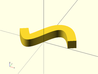
Example 1: A simple sweep of a square along a sine wave:
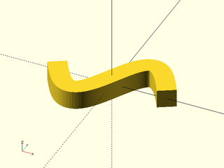
include <BOSL2/std.scad>
path = [for(theta=[-180:5:180]) [theta/10, 10*sin(theta)]];
sq = square(6,center=true);
path_sweep(sq,path);
Example 2: If the square is not centered, then we get a different result because the shape is in a different place relative to the origin:
include <BOSL2/std.scad>
path = [for(theta=[-180:5:180]) [theta/10, 10*sin(theta)]];
sq = square(6);
path_sweep(sq,path);
Example 3: It may not be obvious, but the polyhedron in the previous example is invalid. It will eventually give CGAL errors when you combine it with other shapes. To see this, set profiles to true and look at the left side. The profiles cross each other and intersect. Any time this happens, your polyhedron is invalid, even if it seems to be working at first. Another observation from the profile display is that we have more profiles than needed over a lot of the shape, so if the model is slow, using fewer profiles in the flat portion of the curve might speed up the calculation.
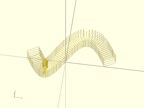
include <BOSL2/std.scad>
path = [for(theta=[-180:5:180]) [theta/10, 10*sin(theta)]];
sq = square(6);
path_sweep(sq,path,profiles=true,width=.1,$fn=8);
Example 4: We'll use this shape in several examples
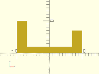
include <BOSL2/std.scad>
ushape = [[-10, 0],[-10, 10],[ -7, 10],[ -7, 2],[  7, 2],[  7, 7],[ 10, 7],[ 10, 0]];
polygon(ushape);
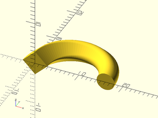
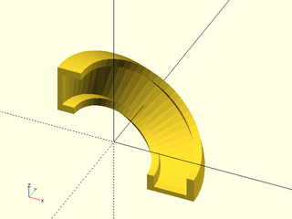
Example 5: Sweep along a clockwise elliptical arc, using default "incremental" method.
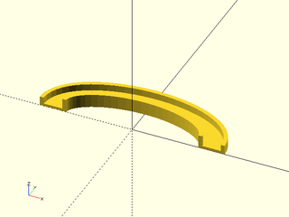
include <BOSL2/std.scad>
ushape = [[-10, 0],[-10, 10],[ -7, 10],[ -7, 2],[  7, 2],[  7, 7],[ 10, 7],[ 10, 0]];
elliptic_arc = xscale(2, p=arc($fn=64,angle=[180,00], r=30));  // Clockwise
path_sweep(ushape, path3d(elliptic_arc));
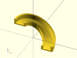
Example 6: Sweep along a counter-clockwise elliptical arc. Note that the orientation of the shape flips.

include <BOSL2/std.scad>
ushape = [[-10, 0],[-10, 10],[ -7, 10],[ -7, 2],[  7, 2],[  7, 7],[ 10, 7],[ 10, 0]];
elliptic_arc = xscale(2, p=arc($fn=64,angle=[0,180], r=30));   // Counter-clockwise
path_sweep(ushape, path3d(elliptic_arc));
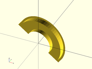
Example 7: Sweep along a clockwise elliptical arc, using "natural" method, which lines up the X axis of the shape with the direction of curvature. This means the X axis will point inward, so a counterclockwise arc gives:
include <BOSL2/std.scad>
ushape = [[-10, 0],[-10, 10],[ -7, 10],[ -7, 2],[  7, 2],[  7, 7],[ 10, 7],[ 10, 0]];
elliptic_arc = xscale(2, p=arc($fn=64,angle=[0,180], r=30));  // Counter-clockwise
path_sweep(ushape, elliptic_arc, method="natural");
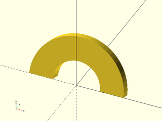
Example 8: Sweep along a clockwise elliptical arc, using "natural" method. If the curve is clockwise then the shape flips upside-down to align the X axis.
include <BOSL2/std.scad>
ushape = [[-10, 0],[-10, 10],[ -7, 10],[ -7, 2],[  7, 2],[  7, 7],[ 10, 7],[ 10, 0]];
elliptic_arc = xscale(2, p=arc($fn=64,angle=[180,0], r=30));  // Clockwise
path_sweep(ushape, path3d(elliptic_arc), method="natural");
Example 9: Sweep along a clockwise elliptical arc, using "manual" method. You can orient the shape in a direction you choose (subject to the constraint that the profiles remain normal to the path):
include <BOSL2/std.scad>
ushape = [[-10, 0],[-10, 10],[ -7, 10],[ -7, 2],[  7, 2],[  7, 7],[ 10, 7],[ 10, 0]];
elliptic_arc = xscale(2, p=arc($fn=64,angle=[180,0], r=30));  // Clockwise
path_sweep(ushape, path3d(elliptic_arc), method="manual", normal=UP+RIGHT);
Example 10: Here we changed the ellipse to be more pointy, and with the same results as above we get a shape with an irregularity in the middle where it maintains the specified direction around the point of the ellipse. If the ellipse were more pointy, this would result in a bad polyhedron:
include <BOSL2/std.scad>
ushape = [[-10, 0],[-10, 10],[ -7, 10],[ -7, 2],[  7, 2],[  7, 7],[ 10, 7],[ 10, 0]];
elliptic_arc = yscale(2, p=arc($fn=64,angle=[180,0], r=30));  // Clockwise
path_sweep(ushape, path3d(elliptic_arc), method="manual", normal=UP+RIGHT);
Example 11: It is easy to produce an invalid shape when your path has a smaller radius of curvature than the width of your shape. The exact threshold where the shape becomes invalid depends on the density of points on your path. The error may not be immediately obvious, as the swept shape appears fine when alone in your model, but adding a cube to the model reveals the problem. In this case the pentagon is turned so its longest direction points inward to create the singularity.
include <BOSL2/std.scad>
qpath = [for(x=[-3:.01:3]) [x,x*x/1.8,0]];
// Prints 0.9, but we use pentagon with radius of 1.0 > 0.9
echo(radius_of_curvature = 1/max(path_curvature(qpath)));
path_sweep(apply(rot(90),pentagon(r=1)), qpath, normal=BACK, method="manual");
cube(0.5);    // Adding a small cube forces a CGAL computation which reveals
              // the error by displaying nothing or giving a cryptic message
Example 12: Using the relax option we allow the profiles to deviate from orthogonality to the path. This eliminates the crease that broke the previous example because the sections are all parallel to each other.
include <BOSL2/std.scad>
qpath = [for(x=[-3:.01:3]) [x,x*x/1.8,0]];
path_sweep(apply(rot(90),pentagon(r=1)), qpath, normal=BACK, method="manual", relaxed=true);
cube(0.5);    // Adding a small cube is not a problem with this valid model
Example 13: Using the profiles=true option can help debug bad polyhedra such as this one. If any of the profiles intersect or cross each other, the polyhedron will be invalid. In this case, you can see these intersections in the middle of the shape, which may give insight into how to fix your shape. The profiles may also help you identify cases with a valid polyhedron where you have more profiles than needed to adequately define the shape.
include <BOSL2/std.scad>
tri= scale([4.5,2.5],[[0, 0], [0, 1], [1, 0]]);
path = left(4,xscale(1.5,arc(r=5,n=25,angle=[-70,70])));
path_sweep(tri,path,profiles=true,width=.1);
Example 14: This 3d arc produces a result that twists to an undefined angle. By default the incremental method sets the starting normal to UP, but the ending normal is unconstrained.
include <BOSL2/std.scad>
ushape = [[-10, 0],[-10, 10],[ -7, 10],[ -7, 2],[  7, 2],[  7, 7],[ 10, 7],[ 10, 0]];
arc = yrot(37, p=path3d(arc($fn=64, r=30, angle=[0,180])));
path_sweep(ushape, arc, method="incremental");
Example 15: You can constrain the last normal as well. Here we point it right, which produces a nice result.
include <BOSL2/std.scad>
ushape = [[-10, 0],[-10, 10],[ -7, 10],[ -7, 2],[  7, 2],[  7, 7],[ 10, 7],[ 10, 0]];
arc = yrot(37, p=path3d(arc($fn=64, r=30, angle=[0,180])));
path_sweep(ushape, arc, method="incremental", last_normal=RIGHT);
Example 16: Here we constrain the last normal to UP. Be aware that the behavior in the middle is unconstrained.
include <BOSL2/std.scad>
ushape = [[-10, 0],[-10, 10],[ -7, 10],[ -7, 2],[  7, 2],[  7, 7],[ 10, 7],[ 10, 0]];
arc = yrot(37, p=path3d(arc($fn=64, r=30, angle=[0,180])));
path_sweep(ushape, arc, method="incremental", last_normal=UP);
Example 17: The "natural" method produces a very different result
include <BOSL2/std.scad>
ushape = [[-10, 0],[-10, 10],[ -7, 10],[ -7, 2],[  7, 2],[  7, 7],[ 10, 7],[ 10, 0]];
arc = yrot(37, p=path3d(arc($fn=64, r=30, angle=[0,180])));
path_sweep(ushape, arc, method="natural");
Example 18: When the path starts at an angle of more that 45 deg to the xy plane the initial normal for "incremental" is BACK. This produces the effect of the shape rising up out of the xy plane. (Using UP for a vertical path is invalid, hence the need for a split in the defaults.)
include <BOSL2/std.scad>
ushape = [[-10, 0],[-10, 10],[ -7, 10],[ -7, 2],[  7, 2],[  7, 7],[ 10, 7],[ 10, 0]];
arc = xrot(75, p=path3d(arc($fn=64, r=30, angle=[0,180])));
path_sweep(ushape, arc, method="incremental");
Example 19: Adding twist
include <BOSL2/std.scad>
// Counter-clockwise
elliptic_arc = xscale(2, p=arc($fn=64,angle=[0,180], r=3));
path_sweep(pentagon(r=1), path3d(elliptic_arc), twist=72);
Example 20: Closed shape
include <BOSL2/std.scad>
ellipse = xscale(2, p=circle($fn=64, r=3));
path_sweep(pentagon(r=1), path3d(ellipse), closed=true);
Example 21: Closed shape with added twist
include <BOSL2/std.scad>
ellipse = xscale(2, p=circle($fn=64, r=3));
// Looks better with finer sampling
pentagon = subdivide_path(pentagon(r=1), 30);
path_sweep(pentagon, path3d(ellipse),
           closed=true, twist=360);
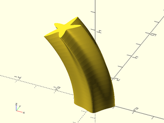
Example 22: The last example was a lot of twist. In order to use less twist you have to tell path_sweep that your shape has symmetry, in this case 5-fold. Mobius strip with pentagon cross section:
include <BOSL2/std.scad>
ellipse = xscale(2, p=circle($fn=64, r=3));
// Looks better with finer sampling
pentagon = subdivide_path(pentagon(r=1), 30);
path_sweep(pentagon, path3d(ellipse), closed=true,
           symmetry = 5, twist=2*360/5);
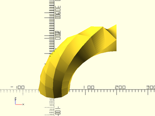
Example 23: A helical path reveals the big problem with the "incremental" method: it can introduce unexpected and extreme twisting. (Note helix example came from list-comprehension-demos)
include <BOSL2/std.scad>
function helix(t) = [(t / 1.5 + 0.5) * 30 * cos(6 * 360 * t),
                     (t / 1.5 + 0.5) * 30 * sin(6 * 360 * t),
                      200 * (1 - t)];
helix_steps = 200;
helix = [for (i=[0:helix_steps]) helix(i/helix_steps)];
ushape = [[-10, 0],[-10, 10],[ -7, 10],[ -7, 2],[  7, 2],[  7, 7],[ 10, 7],[ 10, 0]];
path_sweep(ushape, helix);
Example 24: You can constrain both ends, but still the twist remains:
include <BOSL2/std.scad>
function helix(t) = [(t / 1.5 + 0.5) * 30 * cos(6 * 360 * t),
                     (t / 1.5 + 0.5) * 30 * sin(6 * 360 * t),
                      200 * (1 - t)];
helix_steps = 200;
helix = [for (i=[0:helix_steps]) helix(i/helix_steps)];
ushape = [[-10, 0],[-10, 10],[ -7, 10],[ -7, 2],[  7, 2],[  7, 7],[ 10, 7],[ 10, 0]];
path_sweep(ushape, helix, normal=UP, last_normal=UP);
Example 25: Even if you manually guess the amount of twist and remove it, the result twists one way and then the other:
include <BOSL2/std.scad>
function helix(t) = [(t / 1.5 + 0.5) * 30 * cos(6 * 360 * t),
                     (t / 1.5 + 0.5) * 30 * sin(6 * 360 * t),
                      200 * (1 - t)];
helix_steps = 200;
helix = [for (i=[0:helix_steps]) helix(i/helix_steps)];
ushape = [[-10, 0],[-10, 10],[ -7, 10],[ -7, 2],[  7, 2],[  7, 7],[ 10, 7],[ 10, 0]];
path_sweep(ushape, helix, normal=UP, last_normal=UP, twist=360);
Example 26: To get a good result you must use a different method.
include <BOSL2/std.scad>
function helix(t) = [(t / 1.5 + 0.5) * 30 * cos(6 * 360 * t),
                     (t / 1.5 + 0.5) * 30 * sin(6 * 360 * t),
                      200 * (1 - t)];
helix_steps = 200;
helix = [for (i=[0:helix_steps]) helix(i/helix_steps)];
ushape = [[-10, 0],[-10, 10],[ -7, 10],[ -7, 2],[  7, 2],[  7, 7],[ 10, 7],[ 10, 0]];
path_sweep(ushape, helix, method="natural");
Example 27: Note that it may look like the shape above is flat, but the profiles are very slightly tilted due to the nonzero torsion of the curve. If you want as flat as possible, specify it so with the "manual" method:

include <BOSL2/std.scad>
function helix(t) = [(t / 1.5 + 0.5) * 30 * cos(6 * 360 * t),
                     (t / 1.5 + 0.5) * 30 * sin(6 * 360 * t),
                      200 * (1 - t)];
helix_steps = 200;
helix = [for (i=[0:helix_steps]) helix(i/helix_steps)];
ushape = [[-10, 0],[-10, 10],[ -7, 10],[ -7, 2],[  7, 2],[  7, 7],[ 10, 7],[ 10, 0]];
path_sweep(ushape, helix, method="manual", normal=UP);
Example 28: What if you want to angle the shape inward? This requires a different normal at every point in the path:
include <BOSL2/std.scad>
function helix(t) = [(t / 1.5 + 0.5) * 30 * cos(6 * 360 * t),
                     (t / 1.5 + 0.5) * 30 * sin(6 * 360 * t),
                      200 * (1 - t)];
helix_steps = 200;
helix = [for (i=[0:helix_steps]) helix(i/helix_steps)];
normals = [for(i=[0:helix_steps]) [-cos(6*360*i/helix_steps), -sin(6*360*i/helix_steps), 2.5]];
ushape = [[-10, 0],[-10, 10],[ -7, 10],[ -7, 2],[  7, 2],[  7, 7],[ 10, 7],[ 10, 0]];
path_sweep(ushape, helix, method="manual", normal=normals);
Example 29: When using "manual" it is important to choose a normal that works for the whole path, producing a consistent result. Here we have specified an upward normal, and indeed the shape is pointed up everywhere, but two abrupt transitional twists render the model invalid.
include <BOSL2/std.scad>
yzcircle = yrot(90,p=path3d(circle($fn=64, r=30)));
ushape = [[-10, 0],[-10, 10],[ -7, 10],[ -7, 2],[  7, 2],[  7, 7],[ 10, 7],[ 10, 0]];
path_sweep(ushape, yzcircle, method="manual", normal=UP, closed=true);
Example 30: The "natural" method will introduce twists when the curvature changes direction. A warning is displayed.
include <BOSL2/std.scad>
arc1 = path3d(arc(angle=90, r=30));
arc2 = xrot(-90, cp=[0,30],p=path3d(arc(angle=[90,180], r=30)));
two_arcs = path_merge_collinear(concat(arc1,arc2));
ushape = [[-10, 0],[-10, 10],[ -7, 10],[ -7, 2],[  7, 2],[  7, 7],[ 10, 7],[ 10, 0]];
path_sweep(ushape, two_arcs, method="natural");
Example 31: The only simple way to get a good result is the "incremental" method:
include <BOSL2/std.scad>
arc1 = path3d(arc(angle=90, r=30));
arc2 = xrot(-90, cp=[0,30],p=path3d(arc(angle=[90,180], r=30)));
arc3 = apply( translate([-30,60,30])*yrot(90), path3d(arc(angle=[270,180], r=30)));
three_arcs = path_merge_collinear(concat(arc1,arc2,arc3));
ushape = [[-10, 0],[-10, 10],[ -7, 10],[ -7, 2],[  7, 2],[  7, 7],[ 10, 7],[ 10, 0]];
path_sweep(ushape, three_arcs, method="incremental");
Example 32: knot example from list-comprehension-demos, "incremental" method
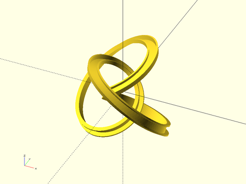
include <BOSL2/std.scad>
function knot(a,b,t) =   // rolling knot
     [ a * cos (3 * t) / (1 - b* sin (2 *t)),
       a * sin( 3 * t) / (1 - b* sin (2 *t)),
     1.8 * b * cos (2 * t) /(1 - b* sin (2 *t))];
a = 0.8; b = sqrt (1 - a * a);
ksteps = 400;
knot_path = [for (i=[0:ksteps-1]) 50 * knot(a,b,(i/ksteps)*360)];
ushape = [[-10, 0],[-10, 10],[ -7, 10],[ -7, 2],[  7, 2],[  7, 7],[ 10, 7],[ 10, 0]];
path_sweep(ushape, knot_path, closed=true, method="incremental");
Example 33: knot example from list-comprehension-demos, "natural" method. Which one do you like better?
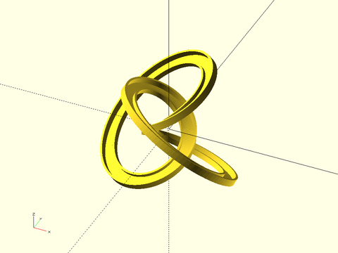
include <BOSL2/std.scad>
function knot(a,b,t) =   // rolling knot
     [ a * cos (3 * t) / (1 - b* sin (2 *t)),
       a * sin( 3 * t) / (1 - b* sin (2 *t)),
     1.8 * b * cos (2 * t) /(1 - b* sin (2 *t))];
a = 0.8; b = sqrt (1 - a * a);
ksteps = 400;
knot_path = [for (i=[0:ksteps-1]) 50 * knot(a,b,(i/ksteps)*360)];
ushape = [[-10, 0],[-10, 10],[ -7, 10],[ -7, 2],[  7, 2],[  7, 7],[ 10, 7],[ 10, 0]];
path_sweep(ushape, knot_path, closed=true, method="natural");
Example 34: knot with twist. Note if you twist it the other direction the center section untwists because of the natural twist there. Also compare to the "incremental" method which has less twist in the center.
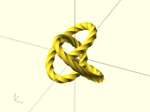
include <BOSL2/std.scad>
function knot(a,b,t) =   // rolling knot
     [ a * cos (3 * t) / (1 - b* sin (2 *t)),
       a * sin( 3 * t) / (1 - b* sin (2 *t)),
     1.8 * b * cos (2 * t) /(1 - b* sin (2 *t))];
a = 0.8; b = sqrt (1 - a * a);
ksteps = 400;
knot_path = [for (i=[0:ksteps-1]) 50 * knot(a,b,(i/ksteps)*360)];
path_sweep(subdivide_path(pentagon(r=12),30), knot_path, closed=true,
           twist=-360*8, symmetry=5, method="natural");
Example 35: twisted knot with twist distributed by path sample points instead of by length using twist_by_length=false

include <BOSL2/std.scad>
function knot(a,b,t) =   // rolling knot
        [ a * cos (3 * t) / (1 - b* sin (2 *t)),
          a * sin( 3 * t) / (1 - b* sin (2 *t)),
        1.8 * b * cos (2 * t) /(1 - b* sin (2 *t))];
a = 0.8; b = sqrt (1 - a * a);
ksteps = 400;
knot_path = [for (i=[0:ksteps-1]) 50 * knot(a,b,(i/ksteps)*360)];
path_sweep(subdivide_path(pentagon(r=12),30), knot_path, closed=true,
           twist=-360*8, symmetry=5, method="natural", twist_by_length=false);
Example 36: This torus knot example comes from list-comprehension-demos. The knot lies on the surface of a torus. When we use the "natural" method the swept figure is angled compared to the surface of the torus because the curve doesn't follow geodesics of the torus.
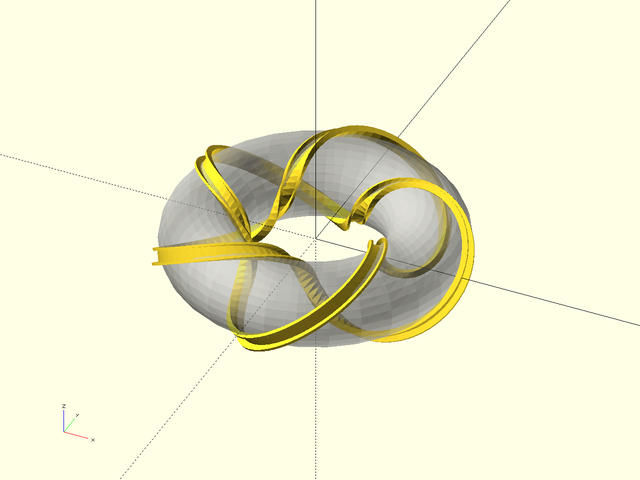
include <BOSL2/std.scad>
function knot(phi,R,r,p,q) =
    [ (r * cos(q * phi) + R) * cos(p * phi),
      (r * cos(q * phi) + R) * sin(p * phi),
       r * sin(q * phi) ];
ushape = 3*[[-10, 0],[-10, 10],[ -7, 10],[ -7, 2],[  7, 2],[  7, 7],[ 10, 7],[ 10, 0]];
points = 50;       // points per loop
R = 400; r = 150;  // Torus size
p = 2;  q = 5;     // Knot parameters
%torus(r_maj=R,r_min=r);
k = max(p,q) / gcd(p,q) * points;
knot_path   = [ for (i=[0:k-1]) knot(360*i/k/gcd(p,q),R,r,p,q) ];
path_sweep(rot(90,p=ushape),knot_path,  method="natural", closed=true);
Example 37: By computing the normal to the torus at the path we can orient the path to lie on the surface of the torus:
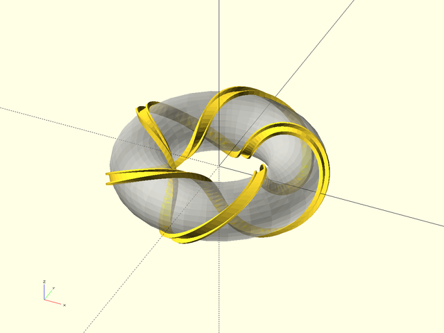
include <BOSL2/std.scad>
function knot(phi,R,r,p,q) =
    [ (r * cos(q * phi) + R) * cos(p * phi),
      (r * cos(q * phi) + R) * sin(p * phi),
       r * sin(q * phi) ];
function knot_normal(phi,R,r,p,q) =
    knot(phi,R,r,p,q)
        - R*unit(knot(phi,R,r,p,q)
            - [0,0, knot(phi,R,r,p,q)[2]]) ;
ushape = 3*[[-10, 0],[-10, 10],[ -7, 10],[ -7, 2],[  7, 2],[  7, 7],[ 10, 7],[ 10, 0]];
points = 50;       // points per loop
R = 400; r = 150;  // Torus size
p = 2;  q = 5;     // Knot parameters
%torus(r_maj=R,r_min=r);
k = max(p,q) / gcd(p,q) * points;
knot_path   = [ for (i=[0:k-1]) knot(360*i/k/gcd(p,q),R,r,p,q) ];
normals = [ for (i=[0:k-1]) knot_normal(360*i/k/gcd(p,q),R,r,p,q) ];
path_sweep(ushape,knot_path,normal=normals, method="manual", closed=true);
Example 38: You can request the transformations and manipulate them before passing them on to sweep. Here we construct a tube that changes scale by first generating the transforms and then applying the scale factor and connecting the inside and outside. Note that the wall thickness varies because it is produced by scaling.
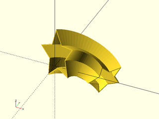
include <BOSL2/std.scad>
shape = star(n=5, r=10, ir=5);
rpath = arc(25, points=[[29,6,-4], [3,4,6], [1,1,7]]);
trans = path_sweep(shape, rpath, transforms=true);
outside = [for(i=[0:len(trans)-1]) trans[i]*scale(lerp(1,1.5,i/(len(trans)-1)))];
inside = [for(i=[len(trans)-1:-1:0]) trans[i]*scale(lerp(1.1,1.4,i/(len(trans)-1)))];
sweep(shape, concat(outside,inside),closed=true);
Example 39: An easier way to scale your model is to use the scale parameter.
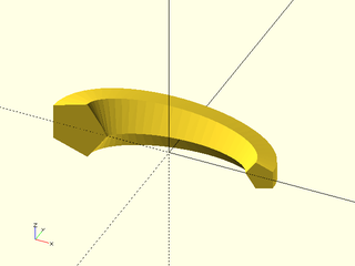
include <BOSL2/std.scad>
elliptic_arc = xscale(2, p=arc($fn=64,angle=[0,180], r=3));
path_sweep(pentagon(r=1), path3d(elliptic_arc), scale=2);
Example 40: Scaling only in the y direction of the profile (z direction in the model in this case)
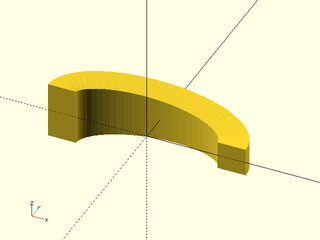
include <BOSL2/std.scad>
elliptic_arc = xscale(2, p=arc($fn=64,angle=[0,180], r=3));
path_sweep(rect(2), path3d(elliptic_arc), scale=[1,2]);
Example 41: Specifying scale at every point for a closed path
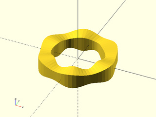
include <BOSL2/std.scad>
N=64;
path = circle(r=5, $fn=64);
theta = lerpn(0,360,N,endpoint=false);
scale = [for(t=theta) sin(6*t)/5+1];
path_sweep(rect(2), path3d(path), closed=true, scale=scale);
Example 42: Using path_sweep on a region
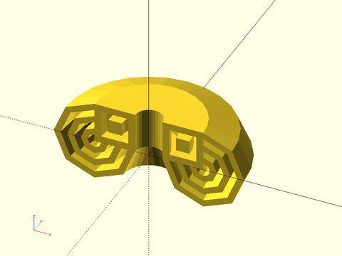
include <BOSL2/std.scad>
rgn1 = [for (d=[10:10:60]) circle(d=d,$fn=8)];
rgn2 = [square(30,center=false)];
rgn3 = [for (size=[10:10:20]) move([15,15],p=square(size=size, center=true))];
mrgn = union(rgn1,rgn2);
orgn = difference(mrgn,rgn3);
path_sweep(orgn,arc(r=40,angle=180));
Example 43: A region with a twist
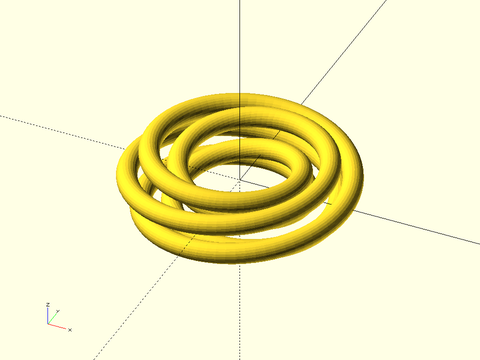
include <BOSL2/std.scad>
region = [for(i=pentagon(5)) move(i,p=circle(r=2,$fn=25))];
path_sweep(region,
           circle(r=16,$fn=75),closed=true,
           twist=360/5*2,symmetry=5);
Example 44: Cutting a cylinder with a curved path. Note that in this case, the incremental method produces just a slight twist but the natural method produces an extreme twist. But manual specification produces no twist, as desired:
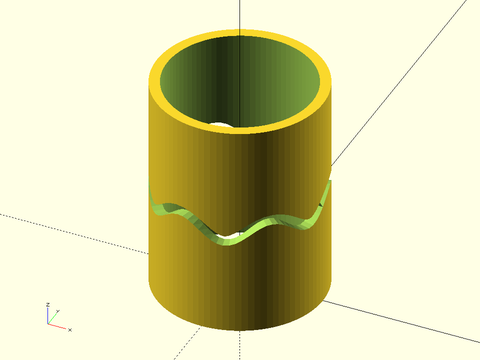
include <BOSL2/std.scad>
$fn=90;
r=8;
thickness=1;
len=21;
curve = [for(theta=[0:4:359])
           [r*cos(theta), r*sin(theta), 10+sin(6*theta)]];
difference(){
  cylinder(r=r, h=len);
  down(.5)cylinder(r=r-thickness, h=len+1);
  path_sweep(left(.05,square([1.1,1])), curve, closed=true,
             method="manual", normal=UP);
}
Example 45: The "start" and "end" anchors are located at the origin point of the swept shape.
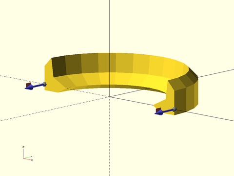
include <BOSL2/std.scad>
shape = back_half(right_half(star(n=5,id=5,od=10)),y=-1);
path = arc(angle=[0,180],d=30);
path_sweep(shape,path,method="natural"){
  attach(["start","end"]) anchor_arrow(s=5);
}
Example 46: The "start" and "end" anchors are located at the origin point of the swept shape.
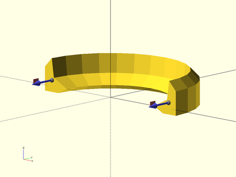
include <BOSL2/std.scad>
shape = back_half(right_half(star(n=5,id=5,od=10)),y=-1);
path = arc(angle=[0,180],d=30);
path_sweep(shape,path,method="natural"){
  attach(["start-centroid","end-centroid"]) anchor_arrow(s=5);
}
Example 47: Note that the "start" anchors are backwards compared to the direction of the sweep, so you have to attach the TOP to align the shape with its ends.
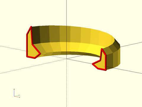
include <BOSL2/std.scad>
shape = back_half(right_half(star(n=5,id=5,od=10)),y=-1)[0];
path = arc(angle=[0,180],d=30);
path_sweep(shape,path,method="natural",scale=[1,1.5])
  recolor("red"){
    attach("start",TOP) stroke([path3d(shape)],width=.5);
    attach("end") stroke([path3d(yscale(1.5,shape))],width=.5);
  }
Synopsis: Sweep a 2d polygon path along a 2d path allowing self-intersection. [VNF] [Geom]
Topics: Extrusion, Sweep, Paths
See Also: linear_sweep(), rotate_sweep(), sweep(), spiral_sweep(), path_sweep(), offset_sweep()
Usage: as module
- path_sweep2d(shape, path, [closed], [caps], [quality], [style], [convexity=], [anchor=], [spin=], [orient=], [atype=], [cp=]) [ATTACHMENTS];
Usage: as function
- vnf = path_sweep2d(shape, path, [closed], [caps], [quality], [style], [anchor=], [spin=], [orient=], [atype=], [cp=]);
Description:
Takes an input 2D polygon (the shape) and a 2d path, and constructs a polyhedron by sweeping the shape along the path. When run as a module returns the polyhedron geometry. When run as a function returns a VNF.
See path_sweep() for more details on how the sweep operation works and for introductory examples.
This 2d version is different because local self-intersections (creases in the output) are allowed and do not produce CGAL errors.
This is accomplished by using offset() calculations, which are more expensive than simply copying the shape along
the path, so if you do not have local self-intersections, use path_sweep() instead. If xmax is the largest x value (in absolute value)
of the shape, then path_sweep2d() will work as long as the offset of path exists at delta=xmax. If the offset vanishes, as in the
case of a circle offset by more than its radius, then you will get an error about a degenerate offset.
Note that global self-intersections will still give rise to CGAL errors. You should be able to handle these by partitioning your model. The y axis of the
shape is mapped to the z axis in the swept polyhedron, and no twisting can occur.
The quality parameter is passed to offset to determine the offset quality.
Arguments:
| By Position | What it does |
|---|---|
shape |
a 2D polygon describing the shape to be swept |
path |
a 2D path giving the path to sweep over |
closed |
path is a closed loop. Default: false |
caps |
true to create endcap faces when closed is false. Can be a length 2 boolean array. Default is true if closed is false. |
quality |
quality of offset used in calculation. Default: 1 |
style |
vnf_vertex_array style. Default: "min_edge" |
| By Name | What it does |
|---|---|
convexity |
convexity parameter for polyhedron (module only) Default: 10 |
anchor |
Translate so anchor point is at the origin. Default: "origin" |
spin |
Rotate this many degrees around Z axis after anchor. Default: 0 |
orient |
Vector to rotate top towards after spin |
atype |
Select "hull" or "intersect" anchor types. Default: "hull" |
cp |
Centerpoint for determining "intersect" anchors or centering the shape. Determintes the base of the anchor vector. Can be "centroid", "mean", "box" or a 3D point. Default: "centroid" |
Anchor Types:
| Anchor Type | What it is |
|---|---|
| "hull" | Anchors to the virtual convex hull of the shape. |
| "intersect" | Anchors to the surface of the shape. |
Example 1: Sine wave example with self-intersections at each peak. This would fail with path_sweep().
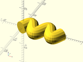
include <BOSL2/std.scad>
sinewave = [for(i=[-30:10:360*2+30]) [i/40,3*sin(i)]];
path_sweep2d(circle(r=3,$fn=15), sinewave);
Example 2: The ends can look weird if they are in a place where self intersection occurs. This is a natural result of how offset behaves at ends of a path.
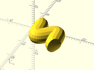
include <BOSL2/std.scad>
coswave = [for(i=[0:10:360*1.5]) [i/40,3*cos(i)]];
zrot(-20)
  path_sweep2d( circle(r=3,$fn=15), coswave);
Example 3: This closed path example works ok as long as the hole in the center remains open.
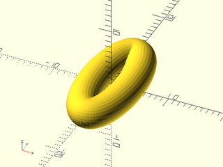
include <BOSL2/std.scad>
ellipse = yscale(3,p=circle(r=3,$fn=120));
path_sweep2d(circle(r=2.5,$fn=32), reverse(ellipse), closed=true);
Example 4: When the hole is closed a global intersection renders the model invalid. You can fix this by taking the union of the two (valid) halves.
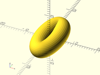
include <BOSL2/std.scad>
ellipse = yscale(3,p=circle(r=3,$fn=120));
L = len(ellipse);
path_sweep2d(circle(r=3.25, $fn=32), select(ellipse,floor(L*.2),ceil(L*.8)),closed=false);
path_sweep2d(circle(r=3.25, $fn=32), select(ellipse,floor(L*.7),ceil(L*.3)),closed=false);
Synopsis: Construct a 3d object from arbitrary transformations of a 2d polygon path. [VNF] [Geom]
Topics: Extrusion, Sweep, Paths
See Also: linear_sweep(), rotate_sweep(), spiral_sweep(), path_sweep(), path_sweep2d(), offset_sweep()
Usage: As Module
- sweep(shape, transforms, [closed], [caps], [style], [convexity=], [anchor=], [spin=], [orient=], [atype=]) [ATTACHMENTS];
Usage: As Function
- vnf = sweep(shape, transforms, [closed], [caps], [style], [anchor=], [spin=], [orient=], [atype=]);
Description:
The input shape must be a non-self-intersecting 2D polygon or region, and transforms
is a list of 4x4 transformation matrices. The sweep algorithm applies each transformation in sequence
to the shape input and links the resulting polygons together to form a polyhedron.
If closed=true then the first and last transformation are linked together.
The caps parameter controls whether the ends of the shape are closed.
As a function, returns the VNF for the polyhedron. As a module, computes the polyhedron.
Note that this is a very powerful, general framework for producing polyhedra. It is important to ensure that your resulting polyhedron does not include any self-intersections, or it will be invalid and will generate CGAL errors. If you get such errors, most likely you have an overlooked self-intersection. Note also that the errors will not occur when your shape is alone in your model, but will arise if you add a second object to the model. This may mislead you into thinking the second object caused a problem. Even adding a simple cube to the model will reveal the problem.
Arguments:
| By Position | What it does |
|---|---|
shape |
2d path or region, describing the shape to be swept. |
transforms |
list of 4x4 matrices to apply |
closed |
set to true to form a closed (torus) model. Default: false |
caps |
true to create endcap faces when closed is false. Can be a singe boolean to specify endcaps at both ends, or a length 2 boolean array. Default is true if closed is false. |
style |
vnf_vertex_array style. Default: "min_edge" |
| By Name | What it does |
|---|---|
convexity |
convexity setting for use with polyhedron. (module only) Default: 10 |
cp |
Centerpoint for determining "intersect" anchors or centering the shape. Determintes the base of the anchor vector. Can be "centroid", "mean", "box" or a 3D point. Default: "centroid" |
atype |
Select "hull" or "intersect" anchor types. Default: "hull" |
anchor |
Translate so anchor point is at the origin. Default: "origin" |
spin |
Rotate this many degrees around Z axis after anchor. Default: 0 |
orient |
Vector to rotate top towards after spin (module only) |
Anchor Types:
| Anchor Type | What it is |
|---|---|
| "hull" | Anchors to the virtual convex hull of the shape. |
| "intersect" | Anchors to the surface of the shape. |
Example 1: A bent object that also changes shape along its length.
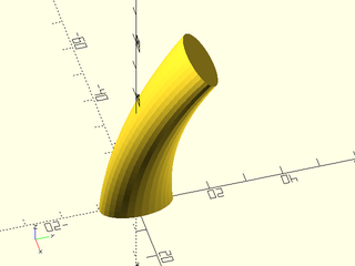
include <BOSL2/std.scad>
radius = 75;
angle = 40;
shape = circle(r=5,$fn=32);
T = [for(i=[0:25]) xrot(-angle*i/25,cp=[0,radius,0])*scale([1+i/25, 2-i/25,1])];
sweep(shape,T);
Example 2: This is the "sweep-drop" example from list-comprehension-demos.
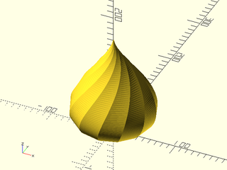
include <BOSL2/std.scad>
function drop(t) = 100 * 0.5 * (1 - cos(180 * t)) * sin(180 * t) + 1;
function path(t) = [0, 0, 80 + 80 * cos(180 * t)];
function rotate(t) = 180 * pow((1 - t), 3);
step = 0.01;
path_transforms = [for (t=[0:step:1-step]) translate(path(t)) * zrot(rotate(t)) * scale([drop(t), drop(t), 1])];
sweep(circle(1, $fn=12), path_transforms);
Example 3: Another example from list-comprehension-demos
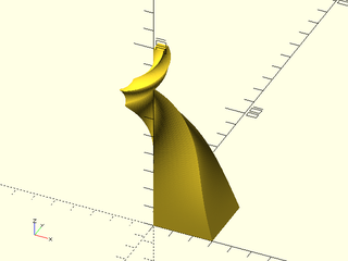
include <BOSL2/std.scad>
function f(x) = 3 - 2.5 * x;
function r(x) = 2 * 180 * x * x * x;
pathstep = 1;
height = 100;
shape_points = subdivide_path(square(10),40,closed=true);
path_transforms = [for (i=[0:pathstep:height]) let(t=i/height) up(i) * scale([f(t),f(t),i]) * zrot(r(t))];
sweep(shape_points, path_transforms);
Example 4: Twisted container. Note that this technique doesn't create a fixed container wall thickness.
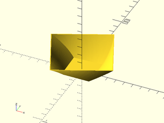
include <BOSL2/std.scad>
shape = subdivide_path(square(30,center=true), 40, closed=true);
outside = [for(i=[0:24]) up(i)*rot(i)*scale(1.25*i/24+1)];
inside = [for(i=[24:-1:2]) up(i)*rot(i)*scale(1.2*i/24+1)];
sweep(shape, concat(outside,inside));
Synopsis: Resample list of paths to have the same point count and interpolate additional paths. [PathList]
Topics: Paths, Path Subdivision
See Also: slice_profiles()
Usage:
- newprof = subdivide_and_slice(profiles, slices, [numpoints], [method], [closed]);
Description:
Subdivides the input profiles to have length numpoints where numpoints must be at least as
big as the largest input profile. By default numpoints is set equal to the length of the
largest profile. You can set numpoints="lcm" to sample to the least common multiple of all
curves, which will avoid sampling artifacts but may produce a huge output. After subdivision,
profiles are sliced.
Arguments:
| By Position | What it does |
|---|---|
profiles |
profiles to operate on |
slices |
number of slices to insert between each pair of profiles. May be a vector |
numpoints |
number of points after sampling. |
method |
method used for calling subdivide_path(), either "length" or "segment". Default: "length"
|
closed |
the first and last profile are connected. Default: false |
Synopsis: Linearly interpolates between path profiles. [PathList]
Topics: Paths, Path Subdivision
See Also: subdivide_and_slice()
Usage:
- profs = slice_profiles(profiles, slices, [closed]);
Description:
Given an input list of profiles, linearly interpolate between each pair to produce a
more finely sampled list. The parameters slices specifies the number of slices to
be inserted between each pair of profiles and can be a number or a list.
Arguments:
| By Position | What it does |
|---|---|
profiles |
list of paths to operate on. They must be lists of the same shape and length. |
slices |
number of slices to insert between each pair, or a list to vary the number inserted. |
closed |
set to true if last profile connects to first one. Default: false |
Synopsis: Resample a list of rotation operators. [MatList]
Topics: Matrices, Interpolation, Rotation
See Also: subdivide_and_slice(), slice_profiles()
Usage:
- rlist = rot_resample(rotlist, n, [method=], [twist=], [scale=], [smoothlen=], [long=], [turns=], [closed=])
Description:
Takes as input a list of rotation matrices in 3d. Produces as output a resampled list of rotation operators (4x4 matrixes) suitable for use with sweep(). You can optionally apply twist to the output with the twist parameter, which is either a scalar to apply a uniform overall twist, or a vector to apply twist non-uniformly. Similarly you can apply scaling either overall or with a vector. The smoothlen parameter applies smoothing to the twist and scaling to prevent abrupt changes. This is done by a moving average of the smoothing or scaling values. The default of 1 means no smoothing. The long parameter causes the interpolation to be done the "long" way around the rotation instead of the short way. Note that the rotation matrix cannot distinguish which way you rotate, only the place you end after rotation. Another ambiguity arises if your rotation is more than 360 degrees. You can add turns with the turns parameter, so giving turns=1 will add 360 degrees to the rotation so it completes one full turn plus the additional rotation given my the transform. You can give long as a scalar or as a vector. Finally if closed is true then the resampling will connect back to the beginning.
The default is to resample based on the length of the arc defined by each rotation operator. This produces uniform sampling over all of the transformations. It requires that each rotation has nonzero length. In this case n specifies the total number of samples. If you set method to "count" then you get n samples for each transform. You can set n to a vector to vary the samples at each step.
Arguments:
| By Position | What it does |
|---|---|
rotlist |
list of rotation operators in 3d to resample |
n |
Number of rotations to produce as output when method is "length" or number for each transformation if method is "count". Can be a vector when method is "count" |
| By Name | What it does |
|---|---|
method |
sampling method, either "length" or "count" |
twist |
scalar or vector giving twist to add overall or at each rotation. Default: none |
scale |
scalar or vector giving scale factor to add overall or at each rotation. Default: none |
smoothlen |
amount of smoothing to apply to scaling and twist. Should be an odd integer. Default: 1 |
long |
resample the "long way" around the rotation, a boolean or list of booleans. Default: false |
turns |
add extra turns. If a scalar adds the turns to every rotation, or give a vector. Default: 0 |
closed |
if true then the rotation list is treated as closed. Default: false |
Example 1: Resampling the arc from a compound rotation with translations thrown in.
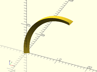
include <BOSL2/std.scad>
tran = rot_resample([ident(4), back(5)*up(4)*xrot(-10)*zrot(-20)*yrot(117,cp=[10,0,0])], n=25);
sweep(circle(r=1,$fn=3), tran);
Example 2: Applying a scale factor
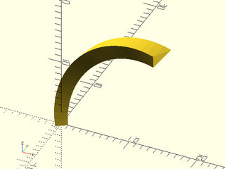
include <BOSL2/std.scad>
tran = rot_resample([ident(4), back(5)*up(4)*xrot(-10)*zrot(-20)*yrot(117,cp=[10,0,0])], n=25, scale=2);
sweep(circle(r=1,$fn=3), tran);
Example 3: Applying twist
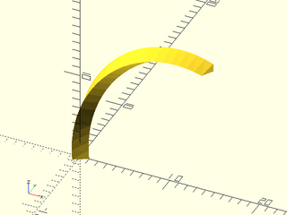
include <BOSL2/std.scad>
tran = rot_resample([ident(4), back(5)*up(4)*xrot(-10)*zrot(-20)*yrot(117,cp=[10,0,0])], n=25, twist=60);
sweep(circle(r=1,$fn=3), tran);
Example 4: Going the long way
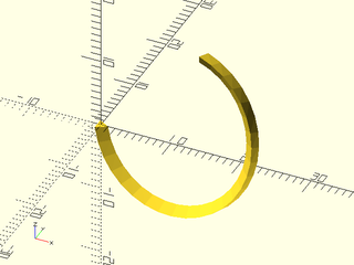
include <BOSL2/std.scad>
tran = rot_resample([ident(4), back(5)*up(4)*xrot(-10)*zrot(-20)*yrot(117,cp=[10,0,0])], n=25, long=true);
sweep(circle(r=1,$fn=3), tran);
Example 5: Getting transformations from turtle3d
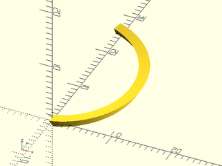
include <BOSL2/std.scad>
include<BOSL2/turtle3d.scad>
tran=turtle3d(["arcsteps",1,"up", 10, "arczrot", 10,170],transforms=true);
sweep(circle(r=1,$fn=3),rot_resample(tran, n=40));
Example 6: If you specify a larger angle in turtle you need to use the long argument
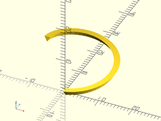
include <BOSL2/std.scad>
include<BOSL2/turtle3d.scad>
tran=turtle3d(["arcsteps",1,"up", 10, "arczrot", 10,270],transforms=true);
sweep(circle(r=1,$fn=3),rot_resample(tran, n=40,long=true));
Example 7: And if the angle is over 360 you need to add turns to get the right result. Note long is false when the remaining angle after subtracting full turns is below 180:
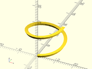
include <BOSL2/std.scad>
include<BOSL2/turtle3d.scad>
tran=turtle3d(["arcsteps",1,"up", 10, "arczrot", 10,90+360],transforms=true);
sweep(circle(r=1,$fn=3),rot_resample(tran, n=40,long=false,turns=1));
Example 8: Here the remaining angle is 270, so long must be set to true
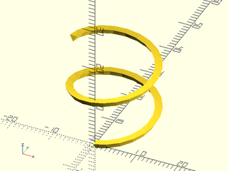
include <BOSL2/std.scad>
include<BOSL2/turtle3d.scad>
tran=turtle3d(["arcsteps",1,"up", 10, "arczrot", 10,270+360],transforms=true);
sweep(circle(r=1,$fn=3),rot_resample(tran, n=40,long=true,turns=1));
Example 9: Note the visible line at the scale transition
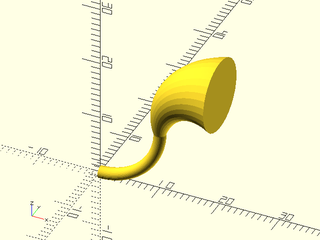
include <BOSL2/std.scad>
include<BOSL2/turtle3d.scad>
tran = turtle3d(["arcsteps",1,"arcup", 10, 90, "arcdown", 10, 90], transforms=true);
rtran = rot_resample(tran,200,scale=[1,6]);
sweep(circle(1,$fn=32),rtran);
Example 10: Observe how using a large smoothlen value eases that transition

include <BOSL2/std.scad>
include<BOSL2/turtle3d.scad>
tran = turtle3d(["arcsteps",1,"arcup", 10, 90, "arcdown", 10, 90], transforms=true);
rtran = rot_resample(tran,200,scale=[1,6],smoothlen=17);
sweep(circle(1,$fn=32),rtran);
Example 11: A similar issues can arise with twist, where a "line" is visible at the transition
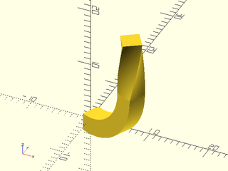
include <BOSL2/std.scad>
include<BOSL2/turtle3d.scad>
tran = turtle3d(["arcsteps", 1, "arcup", 10, 90, "move", 10], transforms=true,state=[1,-.5,0]);
rtran = rot_resample(tran,100,twist=[0,60],smoothlen=1);
sweep(subdivide_path(rect([3,3]),40),rtran);
Example 12: Here's the smoothed twist transition

include <BOSL2/std.scad>
include<BOSL2/turtle3d.scad>
tran = turtle3d(["arcsteps", 1, "arcup", 10, 90, "move", 10], transforms=true,state=[1,-.5,0]);
rtran = rot_resample(tran,100,twist=[0,60],smoothlen=17);
sweep(subdivide_path(rect([3,3]),40),rtran);
Example 13: Toothed belt based on a list-comprehension-demos example. This version has a smoothed twist transition. Try changing smoothlen to 1 to see the more abrupt transition that occurs without smoothing.
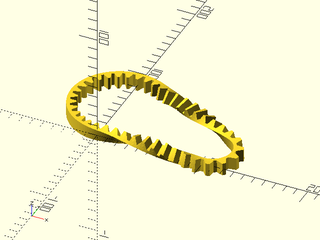
include <BOSL2/std.scad>
include<BOSL2/turtle3d.scad>
r_small = 19;       // radius of small curve
r_large = 46;       // radius of large curve
flat_length = 100;  // length of flat belt section
teeth=42;           // number of teeth
belt_width = 12;
tooth_height = 9;
belt_thickness = 3;
angle = 180 - 2*atan((r_large-r_small)/flat_length);
beltprofile = path3d(subdivide_path(
                square([belt_width, belt_thickness],anchor=FWD),
                20));
beltrots =
  turtle3d(["arcsteps",1,
            "move", flat_length,
            "arcleft", r_small, angle,
            "move", flat_length,
  // Closing path will be interpolated
  //        "arcleft", r_large, 360-angle
           ],transforms=true);
beltpath = rot_resample(beltrots,teeth*4,
                        twist=[180,0,-180,0],
                        long=[false,false,false,true],
                        smoothlen=15,closed=true);
belt = [for(i=idx(beltpath))
          let(tooth = floor((i+$t*4)/2)%2)
          apply(beltpath[i]*
                  yscale(tooth
                         ? tooth_height/belt_thickness
                         : 1),
                beltprofile)
       ];
skin(belt,slices=0,closed=true);
Synopsis: Create vertex association to control how skin() links vertices. [PathList]
Topics: Extrusion, Skinning, Paths
See Also: skin()
Usage:
- newpoly = associate_vertices(polygons, split);
Description:
Takes as input a list of polygons and duplicates specified vertices in each polygon in the list through the series so
that the input can be passed to skin(). This allows you to decide how the vertices are linked up rather than accepting
the automatically computed minimal distance linkage. However, the number of vertices in the polygons must not decrease in the list.
The output is a list of polygons that all have the same number of vertices with some duplicates. You specify the vertex splitting
using the split which is a list where each entry corresponds to a polygon: split[i] is a value or list specifying which vertices in polygon i to split.
Give the empty list if you don't want a split for a particular polygon. If you list a vertex once then it will be split and mapped to
two vertices in the next polygon. If you list it N times then N copies will be created to map to N+1 vertices in the next polygon.
You must ensure that each mapping produces the correct number of vertices to exactly map onto every vertex of the next polygon.
Note that if you split (only) vertex i of a polygon that means it will map to vertices i and i+1 of the next polygon. Vertex 0 will always
map to vertex 0 and the last vertices will always map to each other, so if you want something different than that you'll need to reindex
your polygons.
Arguments:
| By Position | What it does |
|---|---|
polygons |
list of polygons to split |
split |
list of lists of split vertices |
Example 1: If you skin together a square and hexagon using the optimal distance method you get two triangular faces on opposite sides:
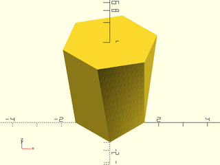
include <BOSL2/std.scad>
sq = regular_ngon(4,side=2);
hex = apply(rot(15),hexagon(side=2));
skin([sq,hex], slices=10, refine=10, method="distance", z=[0,4]);
Example 2: Using associate_vertices you can change the location of the triangular faces. Here they are connect to two adjacent vertices of the square:
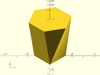
include <BOSL2/std.scad>
sq = regular_ngon(4,side=2);
hex = apply(rot(15),hexagon(side=2));
skin(associate_vertices([sq,hex],[[1,2]]), slices=10, refine=10, sampling="segment", z=[0,4]);
Example 3: Here the two triangular faces connect to a single vertex on the square. Note that we had to rotate the hexagon to line them up because the vertices match counting forward, so in this case vertex 0 of the square matches to vertices 0, 1, and 2 of the hexagon.
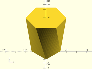
include <BOSL2/std.scad>
sq = regular_ngon(4,side=2);
hex = apply(rot(60),hexagon(side=2));
skin(associate_vertices([sq,hex],[[0,0]]), slices=10, refine=10, sampling="segment", z=[0,4]);
Example 4: This example shows several polygons, with only a single vertex split at each step:
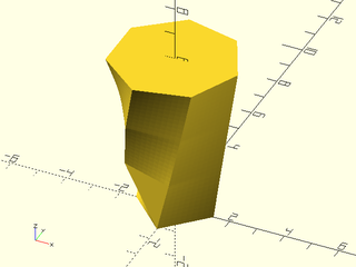
include <BOSL2/std.scad>
sq = regular_ngon(4,side=2);
pent = pentagon(side=2);
hex = hexagon(side=2);
sep = regular_ngon(7,side=2);
profiles = associate_vertices([sq,pent,hex,sep], [1,3,4]);
skin(profiles ,slices=10, refine=10, method="distance", z=[0,2,4,6]);
Example 5: The polygons cannot shrink, so if you want to have decreasing polygons you'll need to concatenate multiple results. Note that it is perfectly ok to duplicate a profile as shown here, where the pentagon is duplicated:
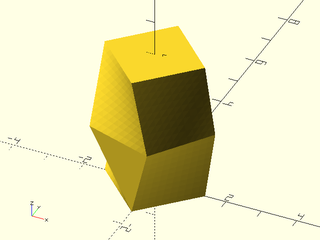
include <BOSL2/std.scad>
sq = regular_ngon(4,side=2);
pent = pentagon(side=2);
grow = associate_vertices([sq,pent], [1]);
shrink = associate_vertices([sq,pent], [2]);
skin(concat(grow, reverse(shrink)), slices=10, refine=10, method="distance", z=[0,2,2,4]);
Some operations are able to add texture to the objects they create. A texture can be any regularly repeated variation in the height of the surface. To define a texture you need to specify how the height should vary over a rectangular block that will be repeated to tile the object. Because textures are based on rectangular tiling, this means adding textures to curved shapes may result in distortion of the basic texture unit. For example, if you texture a cone, the scale of the texture will be larger at the wide end of the cone and smaller at the narrower end of the cone.
You can specify a texture using two methods: a height field or a VNF. For each method you also must specify the scale of the texture, which gives the size of the rectangular unit in your object that will correspond to one texture tile. Note that this scale does not preserve aspect ratio: you can stretch the texture as desired.
The simplest way to specify a texture map is to give a 2d array of height values which specify the height of the texture on a grid. Values in the height field should range from 0 to 1. A zero height in the height field corresponds to the height of the surface and 1 the highest point in the texture above the surface being textured.
Figure 1: Here is a 2d texture described by a "grid" that just contains a single row. Such a texture can be used to create ribbing. The texture is [[0, 1, 1, 0]], and the fixture shows three repetitions of the basic texture unit.
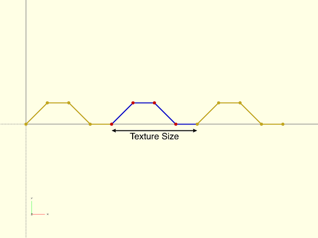
Line segments connect the dots within the texture and also the dots between adjacent texture tiles.
The size of the texture (specified with tex_size) includes the segment that connects the tile to the next one.
Note that the grid is always uniformly spaced.
By default textures are created with unit depth, meaning that the top surface
of the texture is 1 unit above the surface being textured, assuming that the texture
is correctly designed to span the range from 0 to 1. The tex_depth parameter can adjust
this dimension of a texture without changing anything else, and setting tex_depth negative
will invert a texture.
Figure 2:
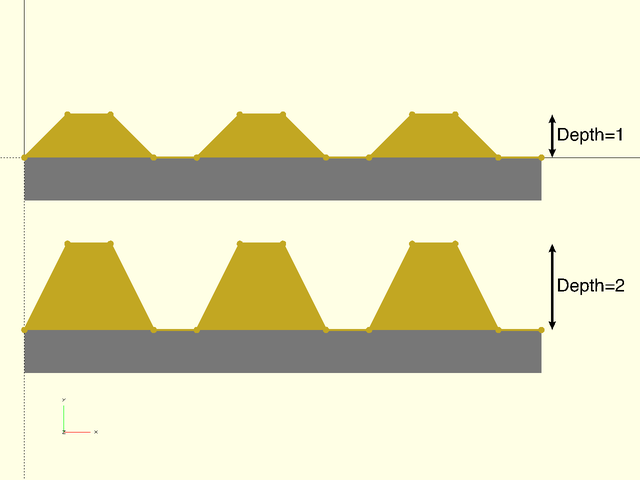
If you want to keep the texture the same size but make the slope
steeper you need to add more points to make the uniform grid fine enough
to represent the slope you want. This means that creating sharp edges
can require a large number of points, resulting in longer run times.
When using the built-in textures you can control the number of points
using the n= argument to texture().
Figure 3:
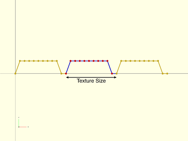
A more serious limitation of height field textures is that some shapes, such as hexagons or circles, cannot be accurately represented because
their points don't fall on any grid. Trying to create such shapes is difficult and will require many points to approximate the
true point positions for the desired shape. This will make the texture slow to compute.
Another serious limitation is more subtle. In the 2D examples above, it is obvious how to connect the
dots together. But in 3D example we need to triangulate the points on a grid, and this triangulation is not unique.
The style argument lets you specify how the points are triangulated using the styles supported by vnf_vertex_array().
In the example below we have expanded the 2D example into 3D:
    [[0,0,0,0],
     [0,1,1,0],
     [0,1,1,0],
     [0,0,0,0]]
and we show the 3D triangulations produced by the different styles:
Figure 4:

Note that of the seven available styles, five produce a different result. There may exist some concave shape where none of the styles produce the right result everywhere on the shape. If this happens it would be another limitation of height field textures. (If you have an example of such a texture and shape please let us know!)
VNF textures overcome all of the limitations of height field textures, but with two costs. They can be more difficult to construct than a simple array of height values, and they are significantly slower to compute for a tile with the same number of points. Note, however, for textures that don't neatly lie on a grid, a VNF tile will be more efficient than a finely sampled height field. With VNF textures you can create textures that have disconnected components, or concavities that cannot be expressed with a single valued height map. However, you can also create invalid textures that fail to close at the ends, so care is required to ensure that your resulting shape is valid.
A VNF texture is defined by defining the texture tile with a VNF whose projection onto the XY plane is contained in the unit square [0,1] x [0,1] so that the VNF can be tiled. The VNF is tiled without a gap, matching the edges, so the vertices along corresponding edges must match to make a consistent triangulation possible. The VNF cannot have any X or Y values outside the interval [0,1]. If you want a valid polyhedron that OpenSCAD will render then you need to take care with edges of the tiles that correspond to endcap faces in the textured object. So for example, in a linear sweep, the top and bottom edges of tiles end abruptly to form the end cap of the object. You can make a valid object in two ways. One way is to create a tile with a single, complete edge along Y=0, and of course a corresponding edges along Y=1. The second way to make a valid object is to have no points at all on the Y=0 line, and of course none on Y=1. In this case, the resulting texture produces a collection of disconnected objects. Note that the Z coordinates of your tile can be anything, but for the dimensional settings on textures to work intuitively, you should construct your tile so that Z ranges from 0 to 1.
Figure 1: This is the "hexgrid" VNF tile, which creates a hexagonal grid texture, something which doesn't work well with a height field because the edges of the hexagon don't align with the grid. Note how the tile ranges between 0 and 1 in both X, Y and Z. In fact, to get a proper aspect ratio in your final texture you need to use the tex_size parameter to introduct a sqrt(3) scale factor.
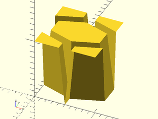
Figure 2: This is an example of a tile that has no edges at the top or bottom, so it creates disconnected rings. See linear_sweep() for examples showing this tile in use.
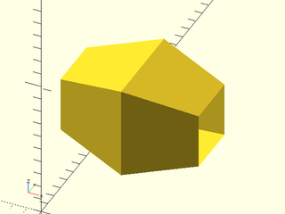
A VNF texture provides a flat structure. In order to apply this structure to a cylinder or other curved object, the VNF must be sliced
and "folded" so it can follow the curve. This folding is controlled by the tex_samples parameter to cyl(), linear_sweep(),
and rotate_sweep(). Note that you specify it when you use the texture, not when you create it. This differs from height
fields, where the analogous parameter is the n= parameter of the texture() function. When tex_samples is too small, only the
points given in the VNF will follow the surface, resulting in a blocky look and geometrical artifacts.
Figure 3: On the left the tex_samples value is small and the texture is blocky. On the right, the default value of 8 allows a reasonable fit to the cylinder.
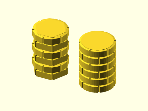
Note that when the VNF is sliced, extra points can be introduced in the interior of faces leading to unexpected irregularities in the textures, which appear as extra triangles. These artifacts can be minimized by making the VNF texture's faces as large as possible rather than using a triangulated VNF, but depending on the specific VNF texture, it may be impossible to entirely eliminate them.
Figure 4: The left shows a normal bricks_vnf texture. The right shows a texture that was first passed through vnf_triangulate(). Note the extra triangle artifacts visible at the ends on the brick faces.
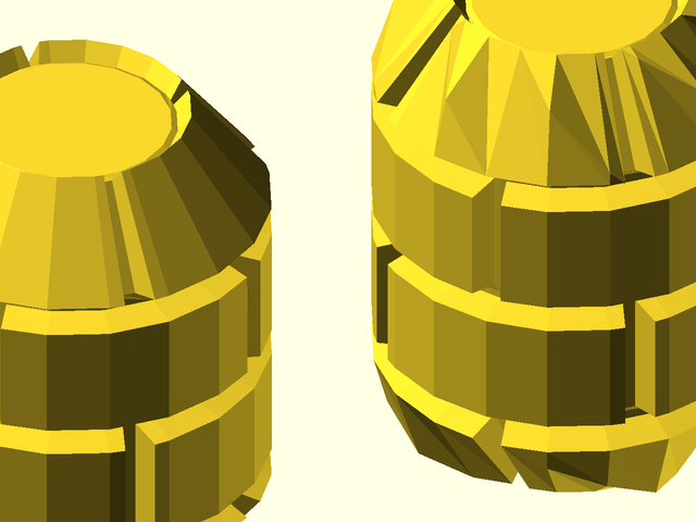
Synopsis: Produce a standard texture.
See Also: linear_sweep(), rotate_sweep(), heightfield(), cylindrical_heightfield()
Usage:
- tx = texture(tex, [n=], [inset=], [gap=], [roughness=]);
Description:
Given a texture name, returns a texture. Textures can come in two varieties:
- Heightfield textures which are 2D arrays of scalars. These are usually faster to render, but can be less precise and prone to triangulation errors. The table below gives the recommended style for the best triangulation. If results are still incorrect, switch to the similar VNF tile by adding the "_vnf" suffix.
- VNF Tile textures, which are VNFs that cover the unit square [0,0] x [1,1]. These tend to be slower to render, but allow greater flexibility and precision for shapes that don't align with a grid.
In the descriptions below, imagine the textures positioned on the XY plane, so "horizontal" refers to the "sideways" dimensions of the texture and "up" and "down" refer to the depth dimension, perpendicular to the surface being textured. If a texture is placed on a cylinder the "depth" will become the radial direction and the "horizontal" direction will be the vertical and tangential directions on the cylindrical surface. All horizontal dimensions for VNF textures are relative to the unit square on which the textures are defined, so a value of 0.25 for a gap or border will refer to 1/4 of the texture's full length and/or width. All supported textures appear below in the examples.
Arguments:
| By Position | What it does |
|---|---|
tex |
The name of the texture to get. |
| By Name | What it does |
|---|---|
n |
The number of samples to use for defining a heightfield texture. Depending on the texture, result will be either n x n or 1 x n. Not allowed for VNF textures. See the tex_samples argument to cyl(), linear_sweep() and rotate_sweep() for controlling the sampling of VNF textures. |
border |
The size of a border region on some VNF tile textures. Generally between 0 and 0.5. |
gap |
The gap between logically distinct parts of some VNF tiles. (ie: gap between bricks, gap between truncated ribs, etc.) |
roughness |
The amount of roughness used on the surface of some heightfield textures. Generally between 0 and 0.5. |
Example 1: "bricks" (Heightfield) = A brick-wall pattern. Giving n= sets the number of heightfield samples to n x n. Default: 24. Giving roughness= adds a level of height randomization to add roughness to the texture. Default: 0.05. Use style="convex".
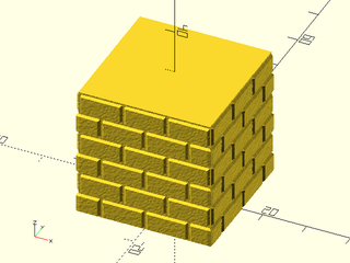
include <BOSL2/std.scad>
tex = texture("bricks");
linear_sweep(
    rect(30), texture=tex, h=30,
    tex_size=[10,10]
);
Example 2: "bricks_vnf" (VNF) = VNF version of "bricks". Giving gap= sets the "mortar" gap between adjacent bricks, default 0.05. Giving border= specifies that the top face of the brick is smaller than the bottom of the brick by border on each of the four sides. If gap is zero then a border value close to 0.5 will cause bricks to come to a sharp pointed edge, with just a tiny flat top surface. Note that gap+border must be strictly smaller than 0.5. Default is border=0.05.
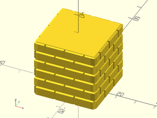
include <BOSL2/std.scad>
tex = texture("bricks_vnf");
linear_sweep(
    rect(30), texture=tex, h=30,
    tex_size=[10,10]
);
Example 3: "bricks_vnf" texture with large border.
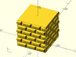
include <BOSL2/std.scad>
tex = texture("bricks_vnf",border=0.25);
linear_sweep(
    rect(30), texture=tex, h=30,
    tex_size=[10,10]
);
Example 4: "checkers" (VNF) = A pattern of alternating checkerboard squares. Giving border= specifies that the top face of the checker surface is smaller than the bottom by border on each of the four sides. As border approaches 0.5 the tops come to sharp corners. You must set border strictly between 0 and 0.5. Default: 0.05.
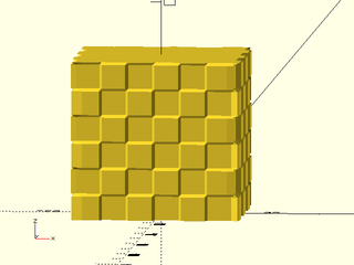
include <BOSL2/std.scad>
tex = texture("checkers");
linear_sweep(
    rect(30), texture=tex, h=30,
    tex_size=[10,10]
);
Example 5: "checkers" texture with large border.
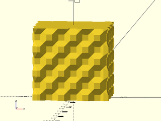
include <BOSL2/std.scad>
tex = texture("checkers",border=0.25);
linear_sweep(
    rect(30), texture=tex, h=30,
    tex_size=[10,10]
);
Example 6: "cones" (VNF) = Raised conical spikes. Specify $fn to set the number of segments on the cone (will be rounded to a multiple of 4). The default is $fn=16. Note that $fa and $fs are ignored, since the scale of the texture is unknown at the time of definition. Giving border= specifies the horizontal border width between the edge of the tile and the base of the cone. The border value must be nonnegative and smaller than 0.5. Default: 0.
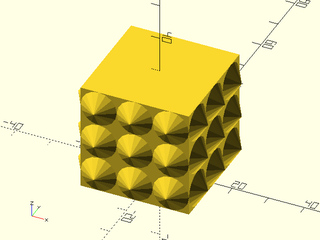
include <BOSL2/std.scad>
tex = texture("cones", $fn=16);
linear_sweep(
    rect(30), texture=tex, h=30, tex_depth=3,
    tex_size=[10,10]
);
Example 7: "cubes" (VNF) = Corner-cubes texture. This texture needs to be scaled in vertically by sqrt(3) to have its correct aspect
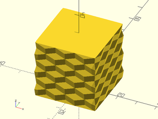
include <BOSL2/std.scad>
tex = texture("cubes");
linear_sweep(
    rect(30), texture=tex, h=30,
    tex_size=[10,10]
);
Example 8: "cubes" texture at the correct scale.
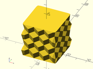
include <BOSL2/std.scad>
tex = texture("cubes");
linear_sweep(
    rect(30), texture=tex, h=20*sqrt(3), tex_depth=3,
    tex_size=[10,10*sqrt(3)]
);
Example 9: "diamonds" (Heightfield) = Four-sided pyramid with the corners of the base aligned with the axes. Compare to "pyramids". Useful for knurling. Giving n= sets the number of heightfield samples to n x n. Default: 2. Use style="concave" for pointed bumps, or style="default" or style="alt" for a diagonal ribs.
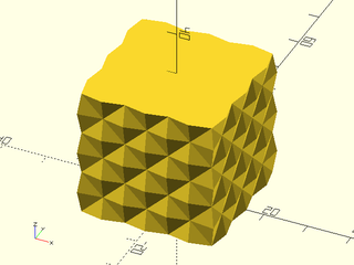
include <BOSL2/std.scad>
tex = texture("diamonds");
linear_sweep(
    rect(30), texture=tex, h=30,
    tex_size=[10,10], style="concave"
);
Example 10: "diamonds" texture can give diagonal ribbing with "default" style.

include <BOSL2/std.scad>
tex = texture("diamonds");
linear_sweep(
    rect(30), texture=tex, h=30,
    tex_size=[10,10], style="default"
);
Example 11: "diamonds" texture gives diagonal ribbing the other direction with "alt" style.
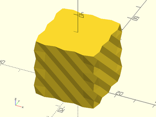
include <BOSL2/std.scad>
tex = texture("diamonds");
linear_sweep(
    rect(30), texture=tex, h=30,
    tex_size=[10,10], style="alt"
);
Example 12: "diamonds_vnf" (VNF) = VNF version of "diamonds".

include <BOSL2/std.scad>
tex = texture("diamonds_vnf");
linear_sweep(
    rect(30), texture=tex, h=30,
    tex_size=[10,10]
);
Example 13: "dimples" (VNF) = Round divots. Specify $fn to set the number of segments on the dimples (will be rounded to a multiple of 4). The default is $fn=16. Note that $fa and $fs are ignored, since the scale of the texture is unknown at the time of definition. Giving border= specifies the horizontal width of the flat border region between the tile edges and the edge of the dimple. Must be nonnegative and strictly less than 0.5. Default: 0.05.
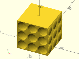
include <BOSL2/std.scad>
tex = texture("dimples", $fn=16);
linear_sweep(
    rect(30), texture=tex, h=30,
    tex_size=[10,10]
);
Example 14: "dots" (VNF) = Raised round bumps. Specify $fn to set the number of segments on the dots (will be rounded to a multiple of 4). The default is $fn=16. Note that $fa and $fs are ignored, since the scale of the texture is unknown at the time of definition. Giving border= specifies the horizontal width of the flat border region between the tile edge and the edge of the dots. Must be nonnegative and strictly less than 0.5. Default: 0.05.
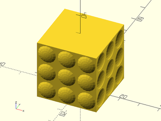
include <BOSL2/std.scad>
tex = texture("dots", $fn=16);
linear_sweep(
    rect(30), texture=tex, h=30,
    tex_size=[10,10]
);
Example 15: "hex_grid" (VNF) = A hexagonal grid defined by V-grove borders. Giving border= specifies that the top face of the hexagon is smaller than the bottom by border on the left and right sides. This means the V-groove top width for grooves running parallel to the Y axis will be double the border value. If the texture is scaled in the Y direction by sqrt(3) then the groove will be uniform on all six sides of the hexagon. Border must be strictly between 0 and 0.5, default: 0.1.

include <BOSL2/std.scad>
tex = texture("hex_grid");
linear_sweep(
    rect(30), texture=tex, h=30,
    tex_size=[10,10]
);
Example 16: "hex_grid" texture with large border
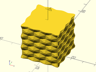
include <BOSL2/std.scad>
tex = texture("hex_grid", border=0.4);
linear_sweep(
    rect(30), texture=tex, h=30,
    tex_size=[10,10]
);
Example 17: "hex_grid" scaled in Y by sqrt(3) so hexagons are regular and grooves are all the same width. Note height of cube is also scaled so tile fits without being automatically adjusted to fit, ruining our choice of scale.
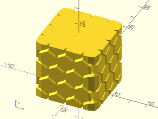
include <BOSL2/std.scad>
tex = texture("hex_grid",border=.07);
linear_sweep(
    rect(30), texture=tex, h=quantup(30,10*sqrt(3)),
    tex_size=[10,10*sqrt(3)], tex_depth=3
);
Example 18: "hex_grid" texture, with approximate scaling because 17 is close to sqrt(3) times 10.
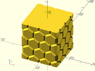
include <BOSL2/std.scad>
tex = texture("hex_grid");
linear_sweep(
    rect(30), texture=tex, h=34,
    tex_size=[10,17]
);
Example 19: "hills" (Heightfield) = Wavy sine-wave hills and valleys, Giving n= sets the number of heightfield samples to n x n. Default: 12. Set style="quincunx".

include <BOSL2/std.scad>
tex = texture("hills");
linear_sweep(
    rect(30), texture=tex, h=30,
    tex_size=[10,10], style="quincunx"
);
Example 20: "pyramids" (Heightfield) = Four-sided pyramid with the edges of the base aligned with the axess. Compare to "diamonds". Useful for knurling. Giving n= sets the number of heightfield samples to n by n. Default: 2. Set style to "convex". Note that style="concave" or style="min_edge" produce mini-diamonds with flat squares in between.

include <BOSL2/std.scad>
tex = texture("pyramids");
linear_sweep(
    rect(30), texture=tex, h=30,
    tex_size=[10,10], style="convex"
);
Example 21: "pyramids" texture, with "concave" produces a mini-diamond texture. Note that "min_edge" also gives this result.
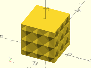
include <BOSL2/std.scad>
tex = texture("pyramids");
linear_sweep(
    rect(30), texture=tex, h=30,
    tex_size=[10,10], style="concave"
);
Example 22: "pyramids_vnf" (VNF) = VNF version of "pyramids".
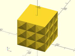
include <BOSL2/std.scad>
tex = texture("pyramids_vnf");
linear_sweep(
    rect(30), texture=tex, h=30,
    tex_size=[10,10]
);
Example 23: "ribs" (Heightfield) = Vertically aligned triangular ribs. Giving n= sets the number of heightfield samples to n by 1. Default: 2. The choice of style does not matter.
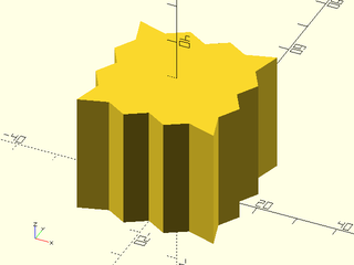
include <BOSL2/std.scad>
tex = texture("ribs");
linear_sweep(
    rect(30), texture=tex, h=30, tex_depth=3,
    tex_size=[10,10], style="concave"
);
Example 24: "rough" (Heightfield) = A pseudo-randomized rough texture. Giving n= sets the number of heightfield samples to n by n. Default: 32. The roughness= parameter specifies the height of the random texture. Default: 0.2.
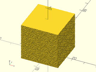
include <BOSL2/std.scad>
tex = texture("rough");
linear_sweep(
    rect(30), texture=tex, h=30,
    tex_size=[10,10], style="min_edge"
);
Example 25: "tri_grid" (VNF) = A triangular grid defined by V-groove borders Giving border= specifies that the top face of the triangular surface is smaller than the bottom by border along the horizontal edges (parallel to the X axis). This means the V-groove top width of the grooves parallel to the X axis will be double the border value. (The other grooves are wider.) If the tile is scaled in the Y direction by sqrt(3) then the groove will be uniform on the three sides of the triangle. The border must be strictly between 0 and 1/6, default: 0.05.
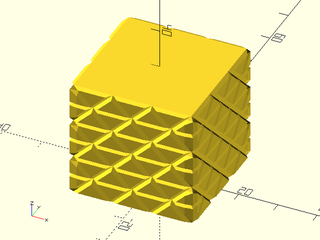
include <BOSL2/std.scad>
tex = texture("tri_grid");
linear_sweep(
    rect(30), texture=tex, h=30,
    tex_size=[10,10]
);
Example 26: "tri_grid" texture with large border. (Max border for tri_grid is 1/6.)
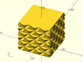
include <BOSL2/std.scad>
tex = texture("tri_grid",border=.12);
linear_sweep(
    rect(30), texture=tex, h=30,
    tex_size=[10,10]
);
Example 27: "tri_grid" texture scaled in Y by sqrt(3) so triangles are equilateral and grooves are all the same width. Note we have to ensure the height evenly fits the scaled texture tiles.
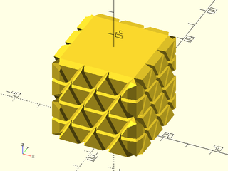
include <BOSL2/std.scad>
tex = texture("tri_grid",border=.04);
linear_sweep(
    rect(30), texture=tex, h=quantup(30,10*sqrt(3)),
    tex_size=[10,10*sqrt(3)], tex_depth=3
);
Example 28: "tri_grid" texture. Here scale makes Y approximately sqrt(3) larger than X so triangles are close to equilateral.
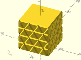
include <BOSL2/std.scad>
tex = texture("tri_grid");
linear_sweep(
    rect(30), texture=tex, h=34,
    tex_size=[10,17]
);
Example 29: "trunc_diamonds" (VNF) = Truncated diamonds, four-sided pyramids with the base corners aligned with the axes and the top cut off. Or you can interpret it as V-groove lines at 45º angles. Giving border= specifies that the width and height of the top surface of the diamond are smaller by border at the left, right, top and bottom. The border is measured in the horizontal direction. This means the V-groove width will be sqrt(2) times the border value. The border must be strictly between 0 and sqrt(2)/4, which is about 0.35. Default: 0.1.

include <BOSL2/std.scad>
tex = texture("trunc_diamonds");
linear_sweep(
    rect(30), texture=tex, h=30,
    tex_size=[10,10]
);
Example 30: "trunc_diamonds" texture with large border.

include <BOSL2/std.scad>
tex = texture("trunc_diamonds",border=.25);
linear_sweep(
    rect(30), texture=tex, h=30,
    tex_size=[10,10]
);
Example 31: "trunc_pyramids" (Heightfield) = Truncated pyramids, four sided pyramids with the base edges aligned to the axes and the top cut off. Giving n= sets the number of heightfield samples to n by n. Default: 6. Set style="convex".
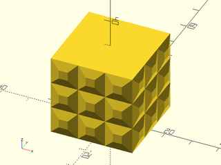
include <BOSL2/std.scad>
tex = texture("trunc_pyramids");
linear_sweep(
    rect(30), texture=tex, h=30,
    tex_size=[10,10], style="convex"
);
Example 32: "trunc_pyramids_vnf" (VNF) = Truncated pyramids, four sided pyramids with the base edges aligned to the axes and the top cut off. You can also regard this as a grid of V-grooves. Giving border= specifies that the top face is smaller than the top by border on all four sides. This means the V-groove top width will be double the border value. The border must be strictly between 0 and 0.5. Default: 0.1.

include <BOSL2/std.scad>
tex = texture("trunc_pyramids_vnf");
linear_sweep(
    rect(30), texture=tex, h=30,
    tex_size=[10,10]
);
Example 33: "trunc_pyramids_vnf" texture with large border
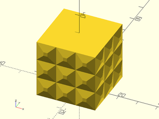
include <BOSL2/std.scad>
tex = texture("trunc_pyramids_vnf", border=.4);
linear_sweep(
    rect(30), texture=tex, h=30,
    tex_size=[10,10]
);
Example 34: "trunc_ribs" (Heightfield) = Truncated ribs. Vertically aligned triangular ribs with the tops cut off, and with rib separation equal to the width of the flat tops. Giving n= sets the number of heightfield samples to n by 1. Default: 4. The style does not matter.
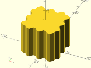
include <BOSL2/std.scad>
tex = texture("trunc_ribs");
linear_sweep(
    rect(30), h=30, texture=tex,
    tex_depth=3, tex_size=[10,10],
    style="concave"
);
Example 35: "trunc_ribs_vnf" (VNF) = Vertically aligned triangular ribs with the tops cut off. Giving gap= sets the bottom gap between ribs. Giving border= specifies that the top rib face is smaller than its base by border on both the left and right sides. The gap measures the flat part between ribs and the border the width of the sloping portion. In order to fit, gap+2*border must be less than 1. (This is because the gap is counted once but the border counts on both sides.) Defaults: gap=1/4, border=1/4.

include <BOSL2/std.scad>
tex = texture("trunc_ribs_vnf", gap=0.25, border=1/6);
linear_sweep(
    rect(30), h=30, texture=tex,
    tex_depth=3, tex_size=[10,10]
);
Example 36: "wave_ribs" (Heightfield) = Vertically aligned wavy ribs. Giving n= sets the number of heightfield samples to n by 1. Default: 8. The style does not matter.
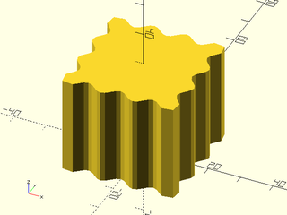
include <BOSL2/std.scad>
tex = texture("wave_ribs");
linear_sweep(
    rect(30), h=30, texture=tex,
    tex_size=[10,10], tex_depth=3, style="concave"
);