Tutorial Paths
A number of advanced features in BOSL2 rely on paths, which are just ordered lists of points.
First-off, some terminology:
- A 2D point is a vector of X and Y axis position values. ie:
[3,4]or[7,-3]. - A 3D point is a vector of X, Y and Z axis position values. ie:
[3,4,2]or[-7,5,3]. - A 2D path is simply a list of two or more 2D points. ie:
[[5,7], [1,-5], [-5,6]] - A 3D path is simply a list of two or more 3D points. ie:
[[5,7,-1], [1,-5,3], [-5,6,1]] - A polygon is a 2D (or planar 3D) path where the last point is assumed to connect to the first point.
- A region is a list of 2D polygons, where each polygon is XORed against all the others. ie: if one polygon is inside another, it makes a hole in the first polygon.
A path can be hard to visualize, since it's just a bunch of numbers in the source code.
One way to see the path is to pass it to polygon():
include <BOSL2/std.scad>
path = [[0,0], [-10,10], [0,20], [10,20], [10,10]];
polygon(path);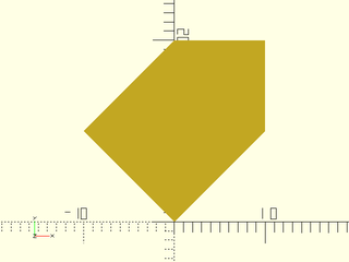
Sometimes, however, it's easier to see just the path itself. For this, you can use the stroke() module.
At its most basic, stroke() just shows the path's line segments:
include <BOSL2/std.scad>
path = [[0,0], [-10,10], [0,20], [10,20], [10,10]];
stroke(path);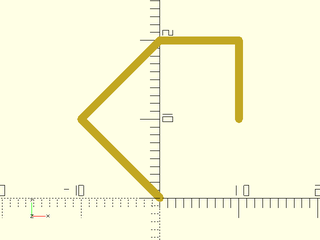
You can vary the width of the drawn path with the width= argument:
include <BOSL2/std.scad>
path = [[0,0], [-10,10], [0,20], [10,20], [10,10]];
stroke(path, width=3);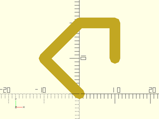
You can vary the line length along the path by giving a list of widths, one per point:
include <BOSL2/std.scad>
path = [[0,0], [-10,10], [0,20], [10,20], [10,10]];
stroke(path, width=[3,2,1,2,3]);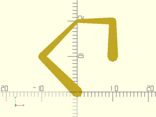
If a path is meant to represent a closed polygon, you can use closed=true to show it that way:
include <BOSL2/std.scad>
path = [[0,0], [-10,10], [0,20], [10,20], [10,10]];
stroke(path, closed=true);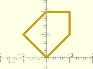
The ends of the drawn path are normally capped with a "round" endcap, but there are other options:
include <BOSL2/std.scad>
path = [[0,0], [-10,10], [0,20], [10,20], [10,10]];
stroke(path, endcaps="round");
include <BOSL2/std.scad>
path = [[0,0], [-10,10], [0,20], [10,20], [10,10]];
stroke(path, endcaps="butt");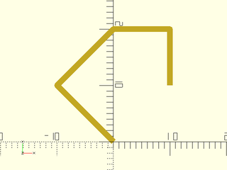
include <BOSL2/std.scad>
path = [[0,0], [-10,10], [0,20], [10,20], [10,10]];
stroke(path, endcaps="line");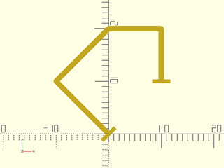
include <BOSL2/std.scad>
path = [[0,0], [-10,10], [0,20], [10,20], [10,10]];
stroke(path, endcaps="tail");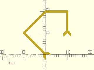
include <BOSL2/std.scad>
path = [[0,0], [-10,10], [0,20], [10,20], [10,10]];
stroke(path, endcaps="arrow2");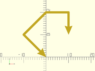
For more standard supported endcap options, see the docs for stroke().
The start and ending endcaps can be specified individually or separately, using endcap1= and endcap2=:
include <BOSL2/std.scad>
path = [[0,0], [-10,10], [0,20], [10,20], [10,10]];
stroke(path, endcap2="arrow2");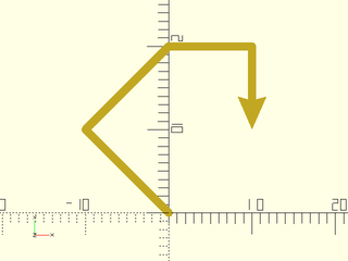
include <BOSL2/std.scad>
path = [[0,0], [-10,10], [0,20], [10,20], [10,10]];
stroke(path, endcap1="butt", endcap2="arrow2");
include <BOSL2/std.scad>
path = [[0,0], [-10,10], [0,20], [10,20], [10,10]];
stroke(path, endcap1="tail", endcap2="arrow");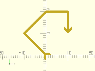
The size of the endcaps will be relative to the width of the line where the endcap is to be placed:
include <BOSL2/std.scad>
path = [[0,0], [-10,10], [0,20], [10,20], [10,10]];
widths = [1, 1.25, 1.5, 1.75, 2];
stroke(path, width=widths, endcaps="arrow2");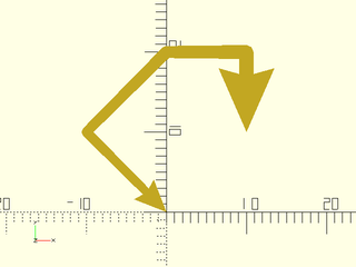
If none of the standard endcaps are useful to you, it is possible to design your own, simply by
passing a path to the endcaps=, endcap1=, or endcap2= arguments. You may also need to give
trim= to tell it how far back to trim the main line, so it renders nicely. The values in the
endcap polygon, and in the trim= argument are relative to the line width. A value of 1 is one
line width size.
Untrimmed:
include <BOSL2/std.scad>
path = [[0,0], [-10,10], [0,20], [10,20], [10,10]];
dblarrow = [[0,0], [2,-3], [0.5,-2.3], [2,-4], [0.5,-3.5], [-0.5,-3.5], [-2,-4], [-0.5,-2.3], [-2,-3]];
stroke(path, endcaps=dblarrow);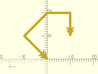
Trimmed:
include <BOSL2/std.scad>
path = [[0,0], [-10,10], [0,20], [10,20], [10,10]];
dblarrow = [[0,0], [2,-3], [0.5,-2.3], [2,-4], [0.5,-3.5], [-0.5,-3.5], [-2,-4], [-0.5,-2.3], [-2,-3]];
stroke(path, trim=3.5, endcaps=dblarrow);
BOSL2 will let you get the perimeter polygon for almost all of the standard 2D shapes simply by calling them like a function:
include <BOSL2/std.scad>
path = square(40, center=true);
stroke(list_wrap(path), endcap2="arrow2");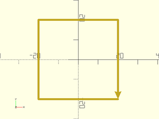
include <BOSL2/std.scad>
path = rect([40,30], rounding=5);
stroke(list_wrap(path), endcap2="arrow2");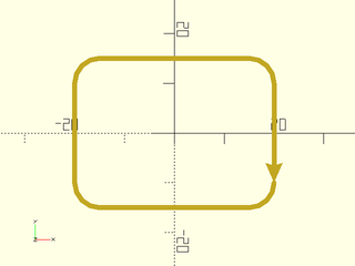
include <BOSL2/std.scad>
path = trapezoid(w1=40, w2=20, h=30);
stroke(list_wrap(path), endcap2="arrow2");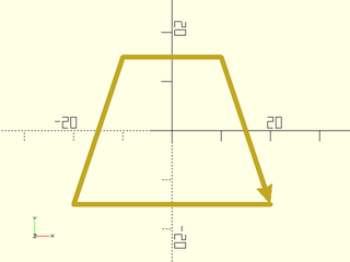
include <BOSL2/std.scad>
path = circle(d=50);
stroke(list_wrap(path), endcap2="arrow2");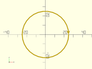
include <BOSL2/std.scad>
path = ellipse(d=[50,30]);
stroke(list_wrap(path), endcap2="arrow2");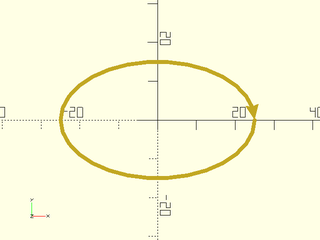
include <BOSL2/std.scad>
path = pentagon(d=50);
stroke(list_wrap(path), endcap2="arrow2");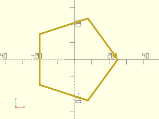
include <BOSL2/std.scad>
path = star(n=5, step=2, d=50);
stroke(list_wrap(path), endcap2="arrow2");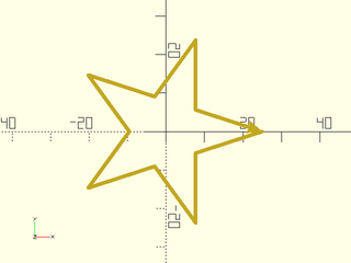
Often, when you are constructing a path, you will want to add an arc. The arc() command lets you do that:
include <BOSL2/std.scad>
path = arc(r=30, angle=120);
stroke(path, endcap2="arrow2");
include <BOSL2/std.scad>
path = arc(d=60, angle=120);
stroke(path, endcap2="arrow2");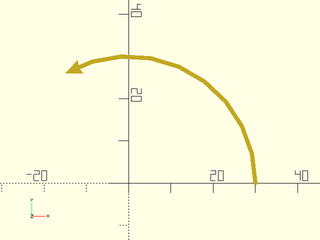
If you give the n= argument, you can control exactly how many points the arc is divided into:
include <BOSL2/std.scad>
path = arc(n=5, r=30, angle=120);
stroke(path, endcap2="arrow2");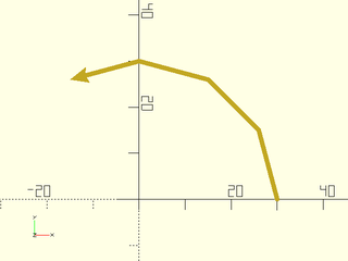
With the start= argument, you can start the arc somewhere other than the X+ axis:
include <BOSL2/std.scad>
path = arc(start=45, r=30, angle=120);
stroke(path, endcap2="arrow2");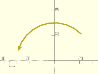
Alternatively, you can give starting and ending angles in a list in the angle= argument:
include <BOSL2/std.scad>
path = arc(angle=[120,45], r=30);
stroke(path, endcap2="arrow2");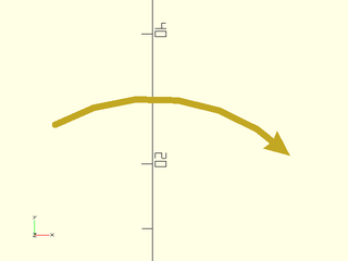
The cp= argument lets you center the arc somewhere other than the origin:
include <BOSL2/std.scad>
path = arc(cp=[10,0], r=30, angle=120);
stroke(path, endcap2="arrow2");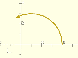
The arc can also be given by three points on the arc:
include <BOSL2/std.scad>
pts = [[-15,10],[0,20],[35,-5]];
path = arc(points=pts);
stroke(path, endcap2="arrow2");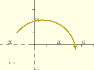
Another way you can create a path is using the turtle() command. It implements a simple path
description language that is similar to LOGO Turtle Graphics. The concept is that you have a virtial
turtle or cursor walking a path. It can "move" forward or backward, or turn "left" or "right" in
place:
include <BOSL2/std.scad>
path = turtle([
    "move", 10,
    "left", 90,
    "move", 20,
    "left", 135,
    "move", 10*sqrt(2),
    "right", 90,
    "move", 10*sqrt(2),
    "left", 135,
    "move", 20
]);
stroke(path, endcap2="arrow2");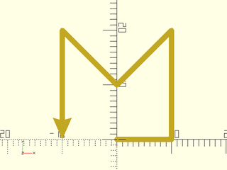
The position and the facing of the turtle/cursor updates after each command. The motion and turning commands can also have default distances or angles given:
include <BOSL2/std.scad>
path = turtle([
    "angle",360/6,
    "length",10,
    "move","turn",
    "move","turn",
    "move","turn",
    "move","turn",
    "move"
]);
stroke(path, endcap2="arrow2");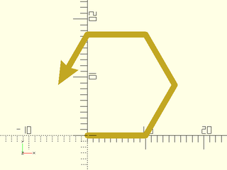
You can use "scale" to relatively scale up the default motion length:
include <BOSL2/std.scad>
path = turtle([
    "angle",360/6,
    "length",10,
    "move","turn",
    "move","turn",
    "scale",2,
    "move","turn",
    "move","turn",
    "scale",0.5,
    "move"
]);
stroke(path, endcap2="arrow2");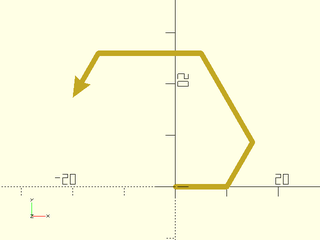
Sequences of commands can be repeated using the "repeat" command:
include <BOSL2/std.scad>
path=turtle([
    "angle",360/5,
    "length",10,
    "repeat",5,["move","turn"]
]);
stroke(path, endcap2="arrow2");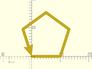
More complicated commands also exist, including those that form arcs:
include <BOSL2/std.scad>
path = turtle([
    "move", 10,
    "left", 90,
    "move", 20,
    "arcleft", 10, 180,
    "move", 20
]);
stroke(path, endcap2="arrow2");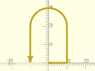
A comprehensive list of supported turtle commands can be found in the docs for turtle().
To translate a path, you can just pass it to the move() (or up/down/left/right/fwd/back) function in the p= argument:
include <BOSL2/std.scad>
path = move([-15,-30], p=square(50,center=true));
stroke(list_wrap(path), endcap2="arrow2");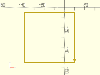
include <BOSL2/std.scad>
path = fwd(30, p=square(50,center=true));
stroke(list_wrap(path), endcap2="arrow2");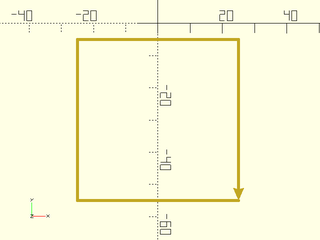
include <BOSL2/std.scad>
path = left(30, p=square(50,center=true));
stroke(list_wrap(path), endcap2="arrow2");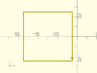
To scale a path, you can just pass it to the scale() (or [xyz]scale) function in the p= argument:
include <BOSL2/std.scad>
path = scale([1.5,0.75], p=square(50,center=true));
stroke(list_wrap(path), endcap2="arrow2");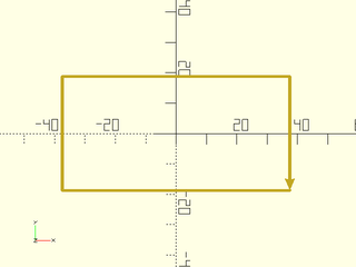
include <BOSL2/std.scad>
path = xscale(1.5, p=square(50,center=true));
stroke(list_wrap(path), endcap2="arrow2");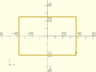
include <BOSL2/std.scad>
path = yscale(1.5, p=square(50,center=true));
stroke(list_wrap(path), endcap2="arrow2");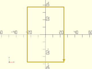
To rotate a path, just can pass it to the rot() (or [xyz]rot) function in the p= argument:
include <BOSL2/std.scad>
path = rot(30, p=square(50,center=true));
stroke(list_wrap(path), endcap2="arrow2");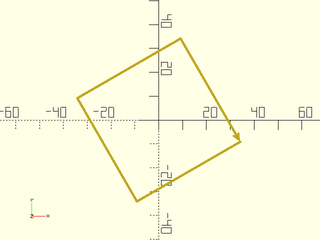
include <BOSL2/std.scad>
path = zrot(30, p=square(50,center=true));
stroke(list_wrap(path), endcap2="arrow2");
To mirror a path, just can pass it to the mirror() (or [xyz]flip) function in the p= argument:
include <BOSL2/std.scad>
path = mirror([1,1], p=trapezoid(w1=40, w2=10, h=25));
stroke(list_wrap(path), endcap2="arrow2");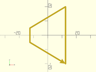
include <BOSL2/std.scad>
path = xflip(p=trapezoid(w1=40, w2=10, h=25));
stroke(list_wrap(path), endcap2="arrow2");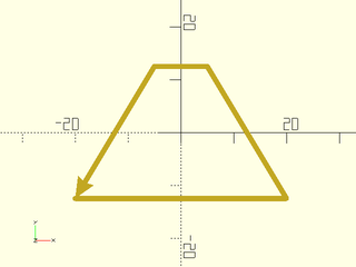
include <BOSL2/std.scad>
path = yflip(p=trapezoid(w1=40, w2=10, h=25));
stroke(list_wrap(path), endcap2="arrow2");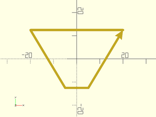
You can get raw transformation matrices for various transformations by calling them like a function without a p= argument:
include <BOSL2/std.scad>
mat = move([5,10,0]);
multmatrix(mat) square(50,center=true);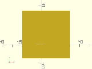
include <BOSL2/std.scad>
mat = scale([1.5,0.75,1]);
multmatrix(mat) square(50,center=true);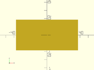
include <BOSL2/std.scad>
mat = rot(30);
multmatrix(mat) square(50,center=true);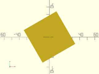
Raw transformation matrices can be multiplied together to precalculate a compound transformation. For example, to scale a shape, then rotate it, then translate the result, you can do something like:
include <BOSL2/std.scad>
mat = move([5,10,0]) * rot(30) * scale([1.5,0.75,1]);
multmatrix(mat) square(50,center=true);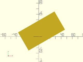
To apply a compound transformation matrix to a path, you can use the apply() function:
include <BOSL2/std.scad>
mat = move([5,10]) * rot(30) * scale([1.5,0.75]);
path = square(50,center=true);
tpath = apply(mat, path);
stroke(tpath, endcap2="arrow2");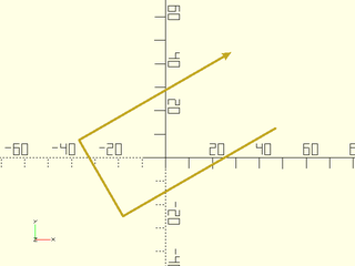
A polygon is good to denote a single closed 2D shape with no holes in it. For more complex 2D
shapes, you will need to use regions. A region is a list of 2D polygons, where each polygon is
XORed against all the others. You can display a region using the region() module.
If you have a region with one polygon fully inside another, it makes a hole:
include <BOSL2/std.scad>
rgn = [square(50,center=true), circle(d=30)];
region(rgn);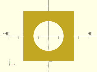
If you have a region with multiple polygons that are not contained by any others, they make multiple discontiguous shapes:
include <BOSL2/std.scad>
rgn = [
    move([-30, 20], p=square(20,center=true)),
    move([  0,-20], p=trapezoid(w1=20, w2=10, h=20)),
    move([ 30, 20], p=square(20,center=true)),
];
region(rgn);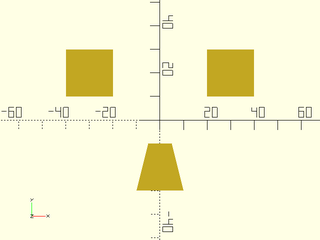
Region polygons can be nested abitrarily deep, in multiple discontiguous shapes:
include <BOSL2/std.scad>
rgn = [
    for (d=[50:-10:10]) left(30, p=circle(d=d)),
    for (d=[50:-10:10]) right(30, p=circle(d=d))
];
region(rgn);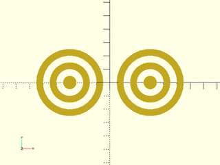
A region with crossing polygons is somewhat poorly formed, but the intersection(s) of the polygons become holes:
include <BOSL2/std.scad>
rgn = [
    left(15, p=circle(d=50)),
    right(15, p=circle(d=50))
];
region(rgn);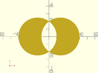
Similarly to how OpenSCAD can perform operations like union/difference/intersection/offset on shape geometry, the BOSL2 library lets you perform those same operations on regions:
include <BOSL2/std.scad>
rgn1 = [for (d=[40:-10:10]) circle(d=d)];
rgn2 = [square([60,12], center=true)];
rgn = union(rgn1, rgn2);
region(rgn);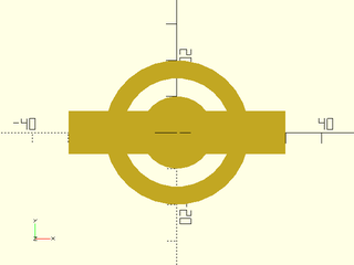
include <BOSL2/std.scad>
rgn1 = [for (d=[40:-10:10]) circle(d=d)];
rgn2 = [square([60,12], center=true)];
rgn = difference(rgn1, rgn2);
region(rgn);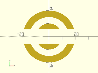
include <BOSL2/std.scad>
rgn1 = [for (d=[40:-10:10]) circle(d=d)];
rgn2 = [square([60,12], center=true)];
rgn = intersection(rgn1, rgn2);
region(rgn);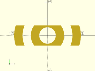
include <BOSL2/std.scad>
rgn1 = [for (d=[40:-10:10]) circle(d=d)];
rgn2 = [square([60,12], center=true)];
rgn = exclusive_or(rgn1, rgn2);
region(rgn);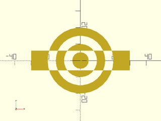
include <BOSL2/std.scad>
orig_rgn = [star(n=5, step=2, d=50)];
rgn = offset(orig_rgn, r=-3, closed=true);
color("blue") region(orig_rgn);
region(rgn);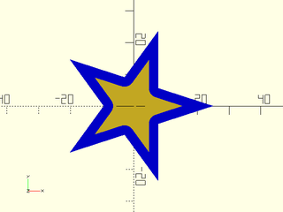
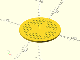
You can use regions for several useful things. If you wanted a grid of holes in your object that
form the shape given by a region, you can do that with grid_copies():
include <BOSL2/std.scad>
rgn = [
    circle(d=100),
    star(n=5,step=2,d=100,spin=90)
];
difference() {
    cyl(h=5, d=120);
    grid_copies(size=[120,120], spacing=[4,4], inside=rgn) cyl(h=10,d=2);
}
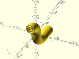
You can also sweep a region through 3-space to make a solid:
include <BOSL2/std.scad>
$fa=1; $fs=1;
rgn = [ for (d=[50:-10:10]) circle(d=d) ];
tforms = [
    for (a=[90:-5:0]) xrot(a, cp=[0,-70]),
    for (a=[0:5:90]) xrot(a, cp=[0,70]),
    move([0,150,-70]) * xrot(90),
];
sweep(rgn, tforms, closed=false, caps=true);