Studio Tutorial: Loading and Viewing the Data - ucdavis/erplab GitHub Wiki
We’re now ready to begin processing the N400 data. To be efficient, the tutorial is limited to data from six carefully selected subjects. We’re going to start by loading and viewing the data from Subject #6 (because this subject’s dataset has some particularly useful properties).
Note that these are not the original ERP CORE data files. The event codes have been shifted slightly to account for the video monitor’s delay, and the channels have been reordered into a more convenient order. Channel location information has also been added.
You should download the data for the tutorial from this link on Box.com: https://ucdavis.app.box.com/v/studio-tutorial. Download the entire folder, which should be named Studio_Tutorial_Files. If you cannot access Box.com, you can try this link on Baidu Cloud Storage (password 1234).
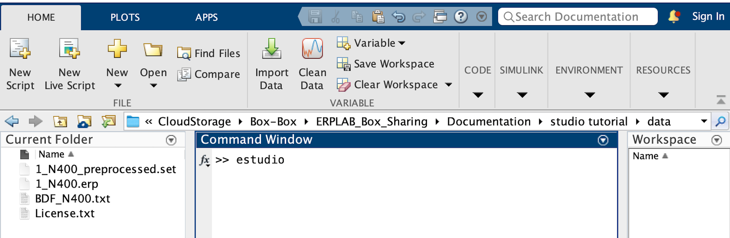
Launch ERPLAB Studio by entering estudio into the Matlab Command Window (followed by Enter or Return). Note that it may take quite a bit of time to launch.
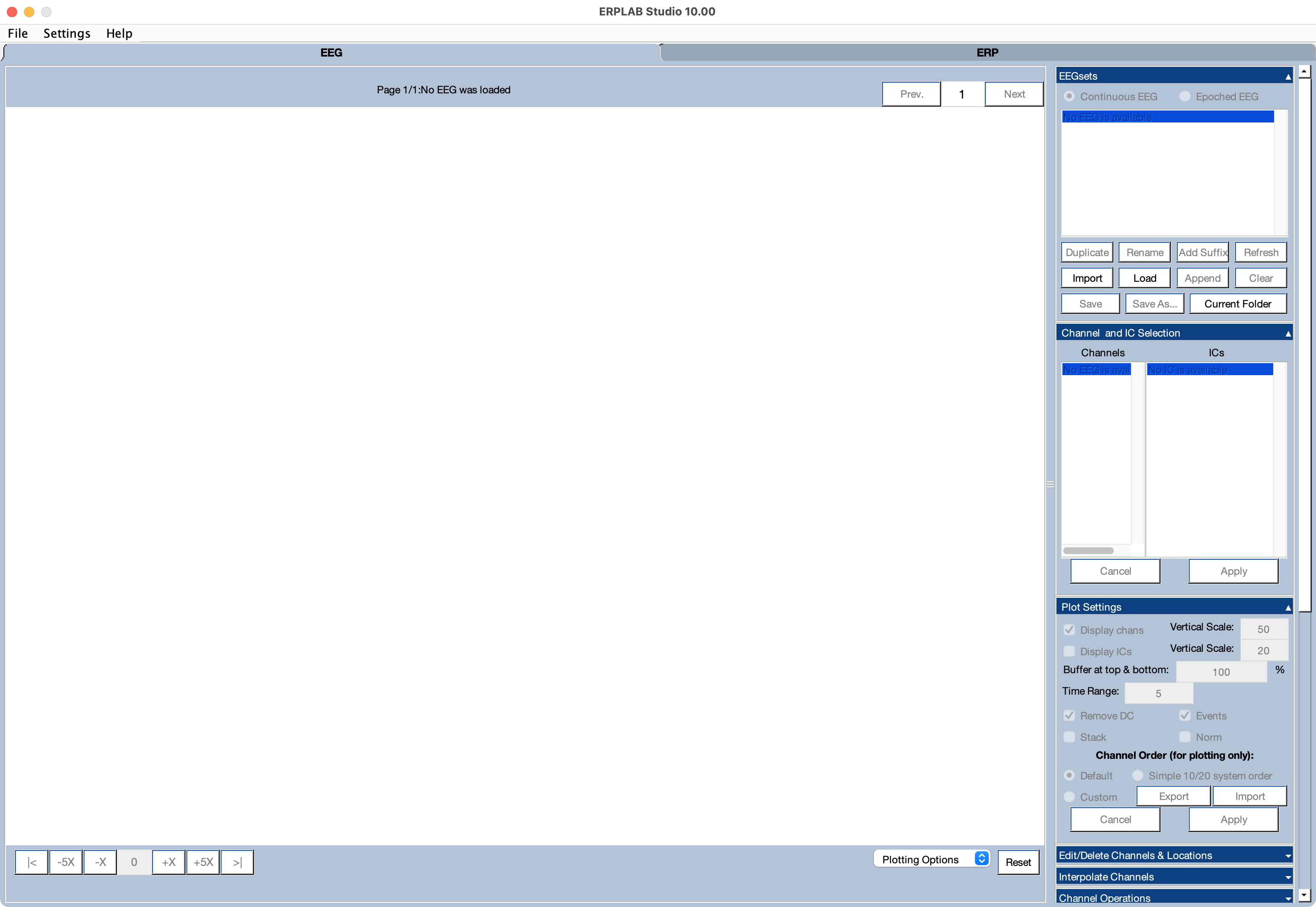
Once the program launches, you will see the main ERPLAB Studio GUI, as shown in the screenshot below. Make sure the EEG tab is selected along the top of the window.
Our next step is to set Matlab’s current folder to be the folder containing the tutorial data, which should be named Studio_Tutorial_Files.
The current folder is part of Matlab’s path, and it’s the first place Matlab will look for files and code. You can set it from ERPLAB Studio by opening the EEGsets panel and clicking Current Folder. Do that now and select the Studio_Tutorial_Files folder that you downloaded in a previous step.
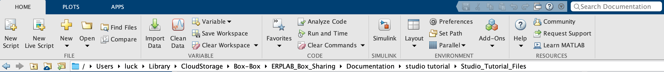
You can also see and change the current folder from the main Matlab window, as shown at the bottom of the following screenshot.
Next we will open the EEG data file from Subject 6. Go to the EEGsets panel and click Load. It should show you all the files in the current folder. Select the one named 6_N400.set.
You should now see the name of that EEGset in the EEGsets panel, the available channels in the Channel and IC Selection panel, and the first 5 seconds of EEG data in the plotting region (see screenshot below). [This EEGset does not contain ICs, which are created when you run independent component analysis, so that list will be empty.]
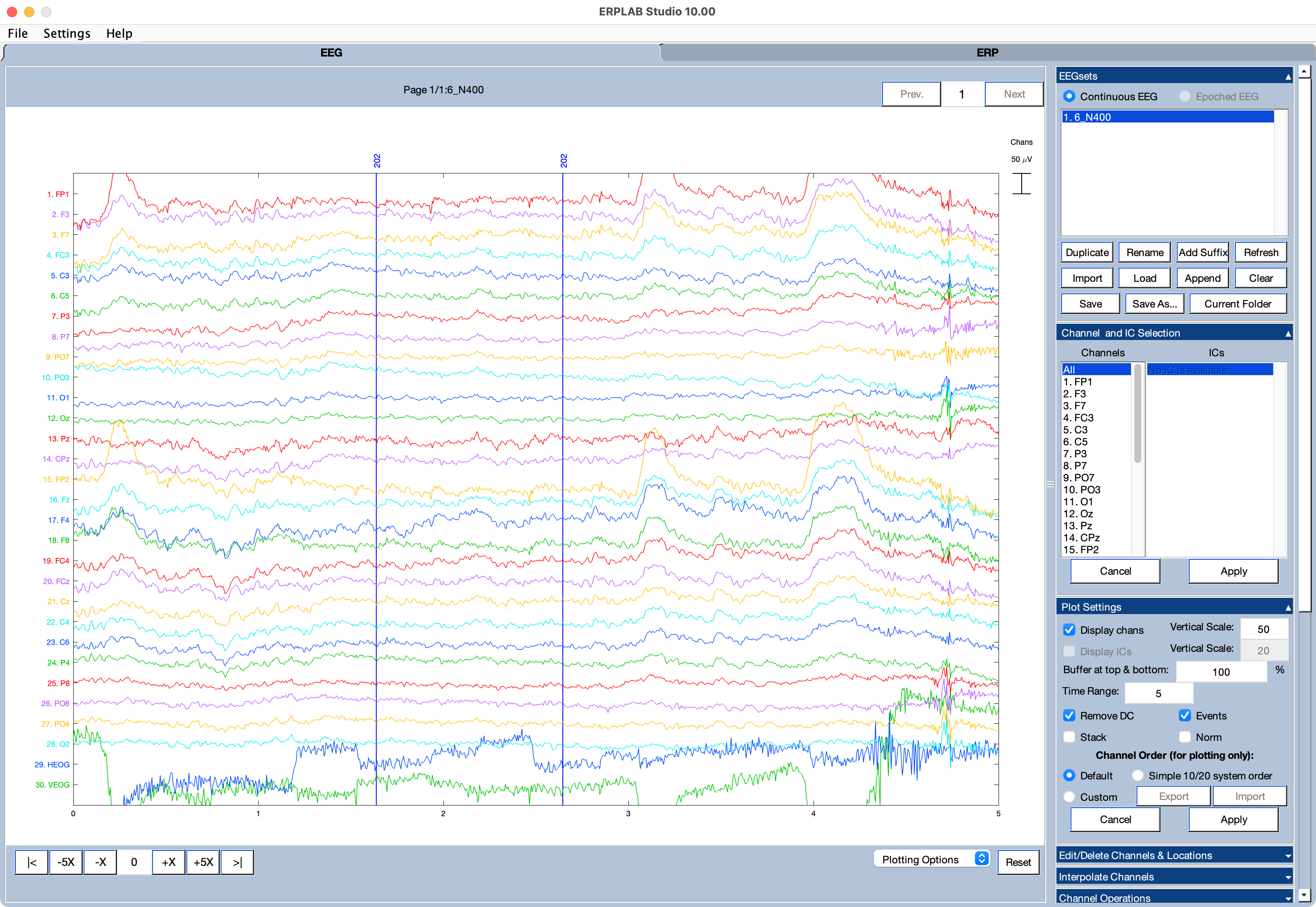
You can scroll through the EEG data by clicking the buttons in the bottom left corner of the plot region. You can enter a number, which will then become the starting point of the plot period (in seconds). The -X and +X buttons shift the plot by one screenful (e.g., by ±5 seconds). The -5X and +5X buttons allow you to shift by 5 screenfuls (e.g., by ±25 seconds). You can also go to the beginning and end with the |< and >| buttons.
You can control which channels are shown by selecting one or more channels in the Channel and IC Selection panel. You can use the Plot Settings panel to control various aspects of the plotting, such as how much time is displayed in each screen (using the Time Range text box) and the vertical scaling (using the Vertical Scale text box).
You can see the event codes as vertical lines with numbers above them in the plotting area. ERPLAB makes no distinction between stimuli, responses, and other types of events (e.g., saccades, heart beats). An event is an event. You get to decide how a given event code is treated in later processing stages (e.g., whether to time-lock to a stimulus or a response, or whether to exclude trials with incorrect responses).
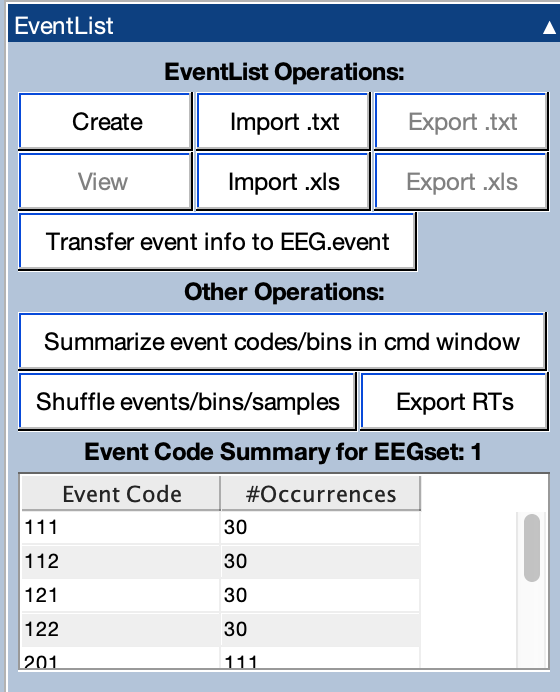
You can see a list of the available event codes and the number of occurrences of each event code by clicking on the EventList panel.
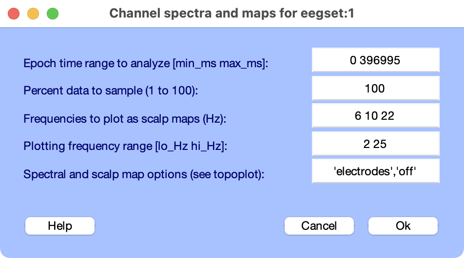
If you’d like to see the frequency content of the EEG, you can apply a Fourier transform to the data and view the spectra. To accomplish this, go to the EEGLAB Tools panel and click on the Spectra & Maps button. This will launch EEGLAB’s tool for plotting EEG spectra. You can just use the default parameters, as shown in the screenshot, and click OK.
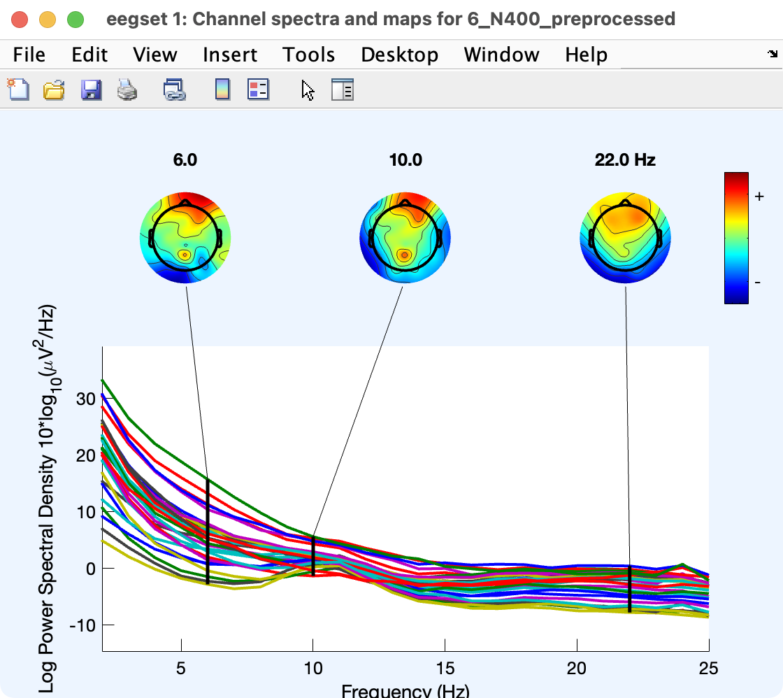
This will generate a spectrum for each channel, and it will show scalp maps for the frequencies that were selected.
Next, we will open the corresponding averaged ERP file from Subject 6 so you can see what it looks like. You will learn how to create averaged ERPs later in the tutorial.
Click on the ERP tab, go to the ERPsets panel and click Load. It should show you all the ERPsets in the current folder. Select the one named 6_N400.erp.
You should now see the name of that ERPset in the ERPsets panel, the available channels and bins in the Channel and Bin Selection panel, and the ERP data in the plotting region (see screenshot below).
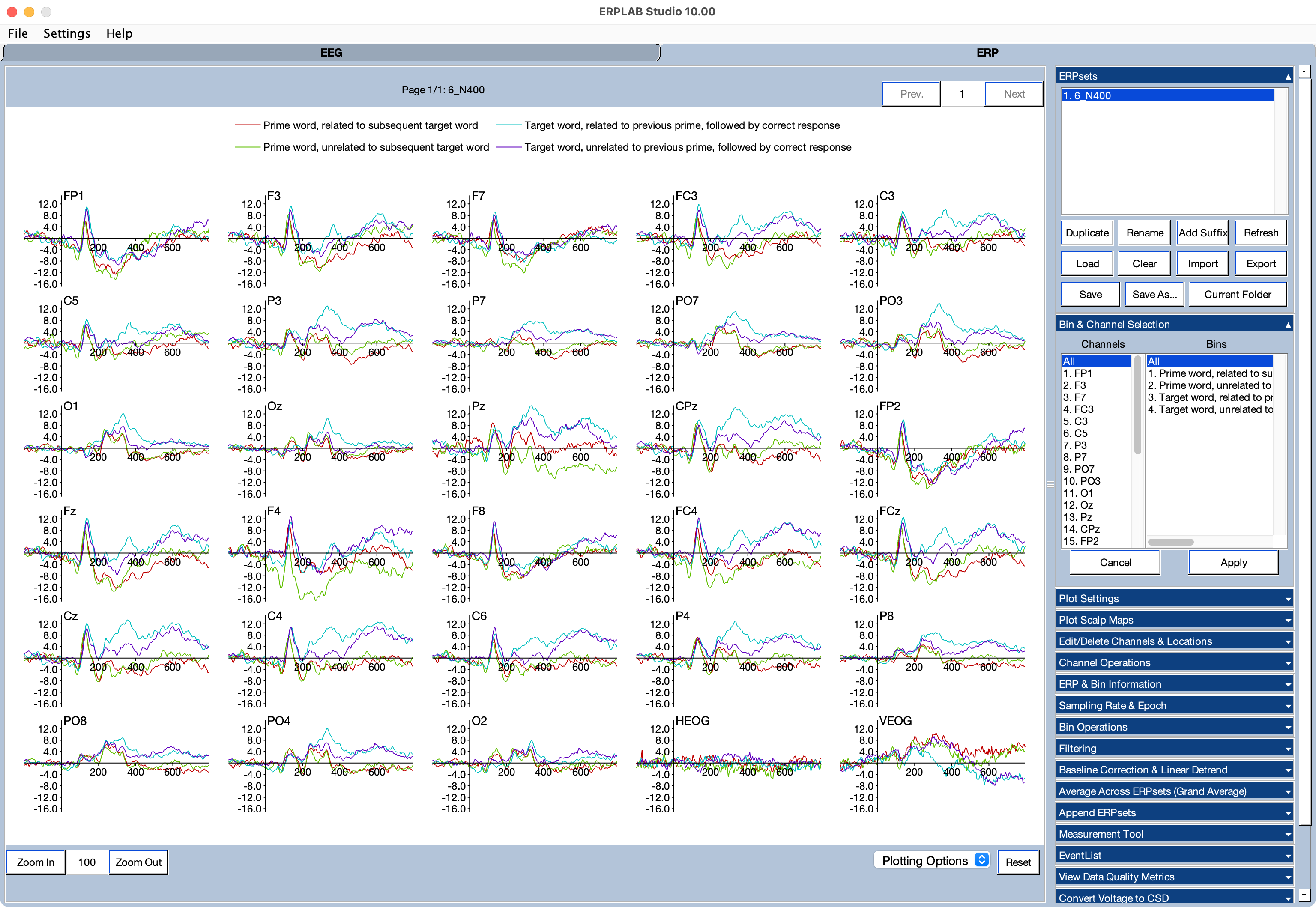
You can control the magnification of the plot by clicking the Zoom In and Zoom Out buttons along the lower left of the plotting region. You can also enter a magnification factor (e.g., 200%) in the box between the Zoom In and Zoom Out buttons.
You can also plot a subset of the channels and bins using the Bin and Channel Selection panel. Try selecting Cz, CPz, and Pz and selecting Bins 3 and 4 as shown in the screenshot.
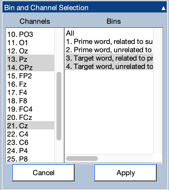
Click Apply to show the data from this set of channels and bins. The result is shown in the screenshot below. You can also select the time range to display, the vertical scale, and other basic plotting parameters in the Plot Settings panel.

The plotting region provides a “quick-and-dirty” view of the waveforms that is very useful while you are processing a subject’s data. To make nicer ERP waveform figures (e.g., for publication), there is an Advanced Waveform Viewer that you can select from the Plotting Options menu at the bottom of the plotting region.
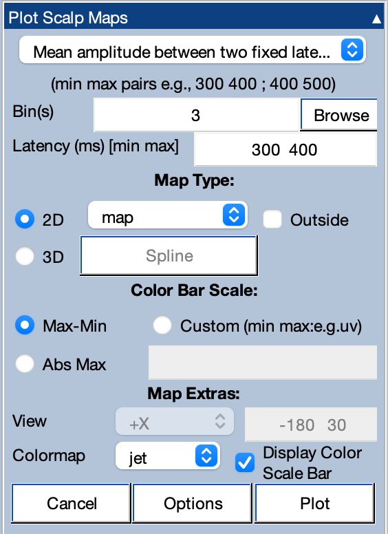
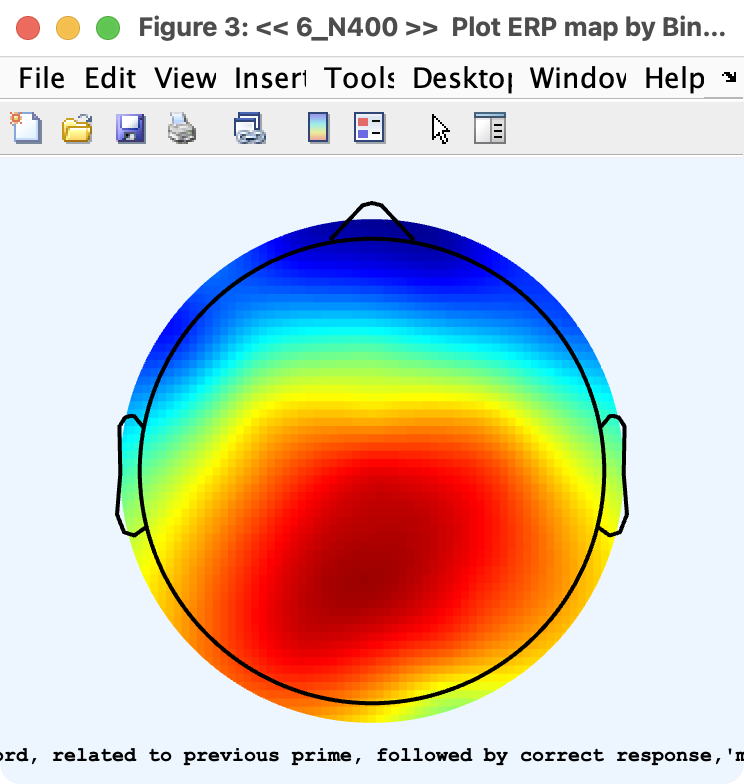
Now let’s see how to plot a scalp map. Go to the Plot Scalp Maps panel, and tell it to plot Bin 3 with a latency range of 300 to 400 ms, as shown in the screenshot. The click Plot, and it will show the scalp distribution of the mean voltage during this latency range.
| Previous Page | Next Page | 🏠 |
|---|---|---|
|
Filtering EEG |
Home |