Studio Tutorial: Artifact Correction and Related Operations - ucdavis/erplab GitHub Wiki
In this tutorial, we will demonstrate ICA-based artifact correction. You can skip this tutorial if you are not interested in using artifact correction. Or you can come back to it later.
Whereas the other tutorial exercises used the data from the ERP CORE N400 experiment, this exercise will use the data from Subject #6 in the mismatch negativity (MMN) experiment (which has useful properties for demonstrating ICA). Chapter 9 of Applied ERP Data Analysis provides more detailed set of examples (using ERPLAB Classic) with Subject #6 and Subject #10 from this experiment.
It is possible to perform ICA-based artifact correction on either epoched EEG or continuous EEG. However, it is usually better to perform it on continuous EEG, and that is what will be demonstrated in this tutorial.
Let’s start by restoring ERPLAB Studio to its default configuration. From the EEG tab, click the Reset button under the lower right corner of the plotting area. You will then see a window that allows you to specify what to reset. Select the option for Restore default parameters for EEG panels and the option for Clear all EEG datasets and click Continue.
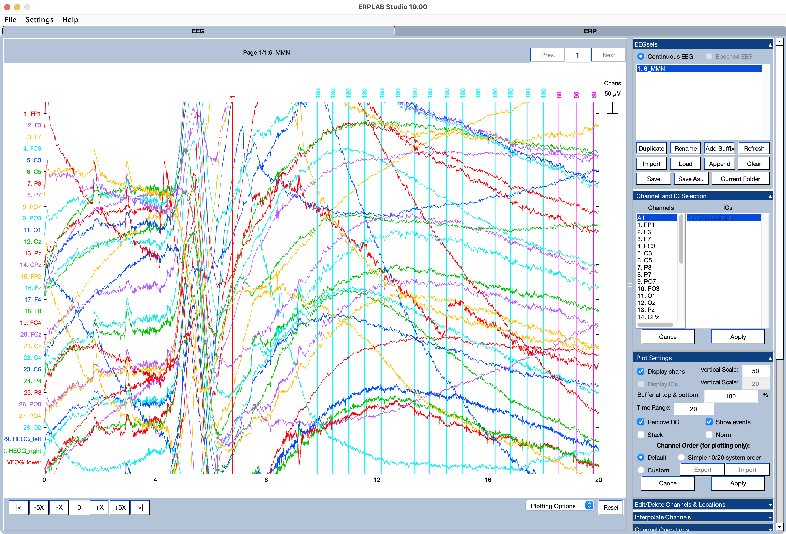
Now go to the EEGsets panel, click Load, and select 6_MMN.set. Then go to the Plot Settings panel and set the Time Range to 20. You should now see something like the screenshot below, with huge artifacts during the first 20 seconds. Scroll through the data, and you will see that there are large low-frequency drifts throughout the recording.
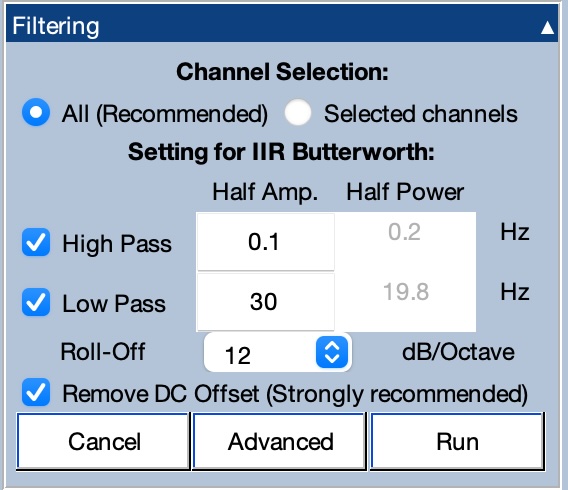
We’re now going to apply a mild bandpass filter to the data by going to the Filtering panel and setting a high-pass cutoff of 0.1 Hz and a low-pass cutoff of 30 Hz (as shown in the screenshot). Save the new EEGset with the name 6_MMN_filt.
You should see that there is still quite a bit of artifact in the first 20 seconds of the filtered data, but you will see much less drifting if you scroll through the data. You will see a lot of blinks in the FP1 and VEOG_lower channels. These extend outside the plotting area, and you can see them better if you go to Plot Settings and change the Buffer at top & bottom from 100 to 200.
An important property of the 6_MMN dataset is that all of the channels have the same reference (the average of P9 and P10). By contrast, the N400 datasets used in the rest of this tutorial have bipolar VEOG and HEOG signals. In the 6_MMN dataset, the VEOG signal is labeled VEOG_lower to indicate that it is a recording from an electrode under the right eye (referenced to the average of P9 and P10). In addition, there are separate HEOG_left and HEOG_right channels, recorded from electrodes to the left and right of the eyes (referenced to the average of P9 and P10).
When you apply ICA, it is usually best to make sure that all channels have the same reference. However, it is also useful to have bipolar channels for the EOG signals so that you can better see the artifacts. Although these two goals appear to conflict, we can achieve both of them by creating additional bipolar VEOG and HEOG channels but then excluding them from the ICA process.
We recommend keeping uncorrected versions of the bipolar EOG signals so you can use them to (a) determine which independent components correspond to artifacts, (b) reject trials for which the eyes were closed or moving at the time of the stimulus, and (c) assess how well the ICA removed the artifacts. You can read Chapter 9 of Applied ERP Data Analysis for the logic behind this recommendation and Zhang et al (2024) for a detailed approach to assessing the effectiveness of ICA.
You will create the bipolar VEOG signal by subtracting the voltage above the eyes (the FP2 channel) from the voltage below the eyes (the VEOG_lower channel). You will create the bipolar HEOG signal by subtracting the voltage to the left of the eyes (the HEOG_left channel) from the voltage to the right of the eyes (the HEOG_right channel).
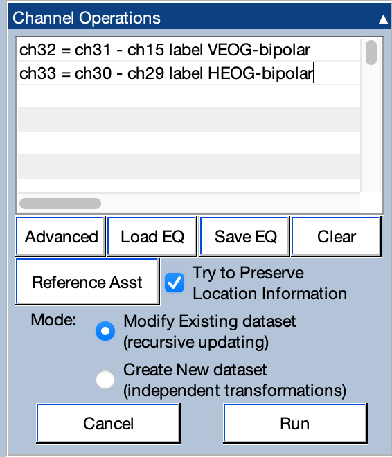
To implement these subtractions, go to the Channel Operations panel, make sure the Mode is set to Modify Existing dataset, and enter these equations as shown in the screenshot:
ch32 = ch31 - ch15 label VEOG-bipolar
ch33 = ch30 - ch29 label HEOG-bipolar
Click Run. You should now see the new bipolar VEOG and HEOG signals at the bottom of the plot window.
Because the Channel Operations tool was run in Modify Existing Dataset mode, it added the new channels to the 6_MMN_filt EEGset rather than creating a new EEGset. However, it would be good for the name to reflect the fact that bipolar EOG channels have been added. To accomplish this, go to the EEGsets panel, click Rename, and enter 6_MMN_filt_bipolar as the New setname (and click Apply). Then click Save and save the EEGset in a file named 6_MMN_filt_bipolar.set.
The next step implements an approach that dramatically improves ICA-based artifact correction in most situations. You can read the justification in Chapter 9 of Applied ERP Data Analysis, but the basic idea is that the process of computing the independent components (called ICs) assumes that each underlying IC has a consistent scalp distribution throughout the recording session. It does not work as well if the EEGset contains large artifacts that do not have a consistent scalp distributions. For example, if the participant stretches during a break or makes a sudden movement that slightly shifts the electrodes, you will get a large artifact that does not have a consistent scalp distribution. We need to minimize these artifacts from the EEGset before computing the ICs (i.e., before performing the ICA decomposition).
Some of these artifacts can be eliminated by deleting short sections of the EEGset that have large and idiosyncratic artifacts (e.g., break periods, brief periods of movement). However, some of these artifacts consist of low-frequency drifts that last a very long time. These latter artifacts can be minimized by applying an extreme high-pass filter (e.g., with a 1 Hz cutoff and a steep roll-off). However, these filters can massively distort the time course of the ERPs and should be avoided in most experiments (see Chapter 7 in An Introduction to the Event-Related Potential Technique; Tanner et al., 2015; and Zhang et al., 2024). Thus, extreme high-pass filtering is helpful for optimizing ICA, but it also has major negative consequences.
To solve this conundrum, we use a trick: We create a special filtered version of the EEGset that we use to perform the ICA decomposition, and then we transfer the IC weights back to the original EEGset that was not subjected to the extreme filtering. We then correct the artifacts in the original EEGset.
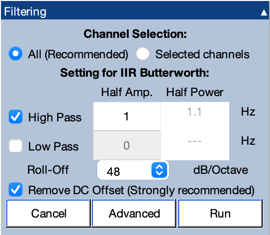
To implement this process, make sure that 6_MMN_filt_bipolar is selected in the EEGsets panel, go to the Filtering panel, and select a high-pass cutoff of 1 Hz with a roll-off of 48 dB/octave (as shown in the screenshot below). Click Run, name the new EEGset 6_MMN_filt_bipolar_extremefilt, and save it to disk as 6_MMN_filt_bipolar_extremefilt.set.
You will see that the huge idiosyncratic artifact during the first 20 seconds has been largely eliminated, and yet you can still see the blink artifacts.
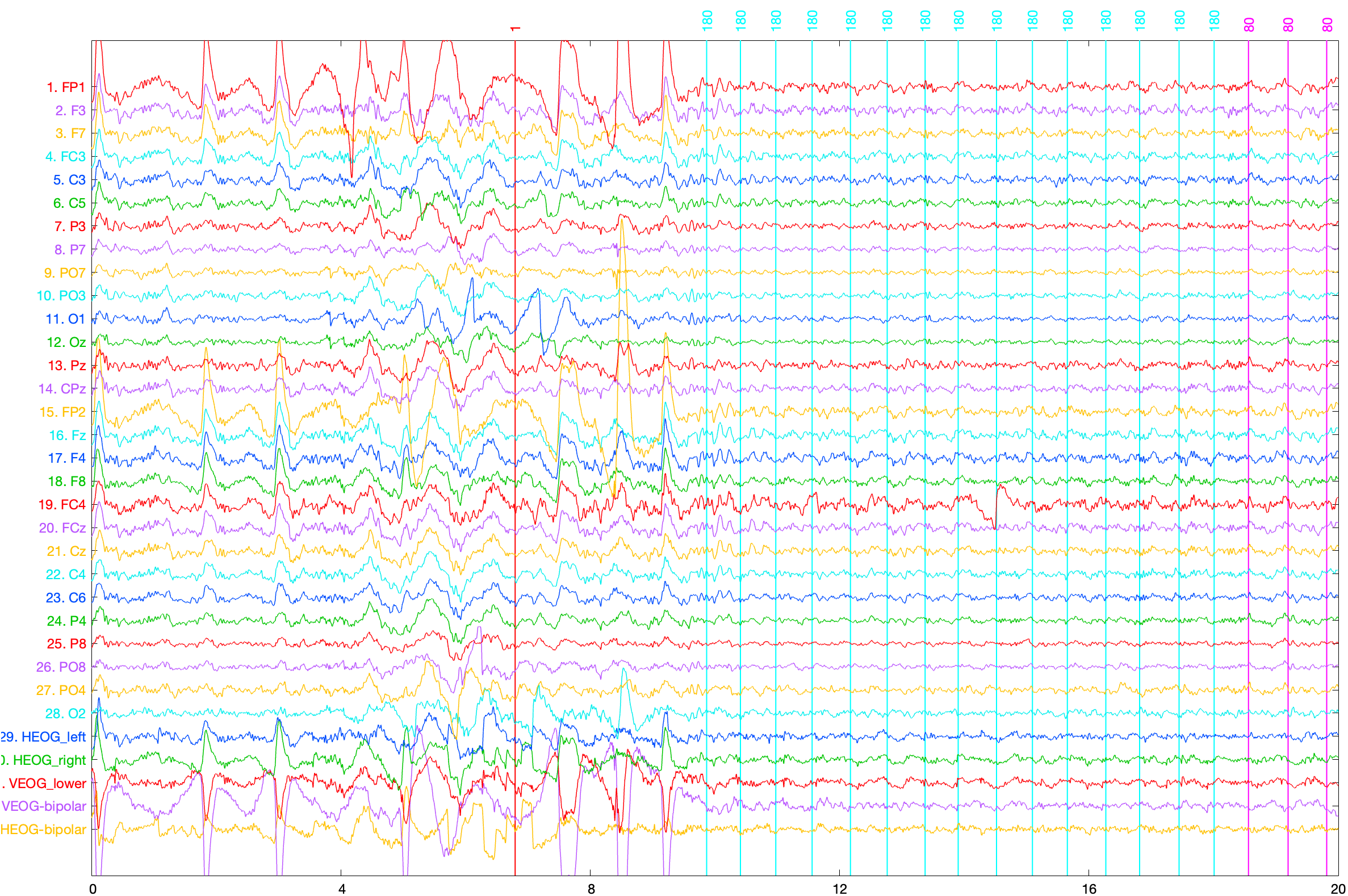
The next step is to delete break periods, when other idiosyncratic artifacts are likely to occur. A break period is defined as a period of time during which no event codes are present. For example, if you look at the first 20 seconds of 6_MMN_filt_bipolar_extremefilt, you can see that a regular stream of event codes begins approximately 10 seconds after the start of the recording.
To delete the break periods from this EEGset, go to the Delete Time Segments panel and set the Time Threshold value to 1500 (see screenshot below). This defines a break as a period of 1500 ms or longer without an event code. (Note that you might need a longer threshold in experiments with slower stimulus presentation rates.)
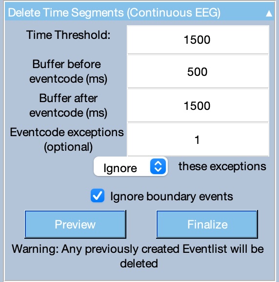
We want to have 500 ms of EEG prior to the first event code after a break, so set Buffer before eventcode to 500. In addition, we want to have 1500 ms of EEG after the last event code prior to a break, so set Buffer after eventcode to 1500.
In this particular experiment, event code 1 occasionally appears during break periods (e.g., the code approximately 7 seconds into the recording). We therefore want to ignore this event code when determining break periods, so enter 1 for Eventcode exceptions. We also want to ignore boundary events that occur during breaks, so check the box for Ignore boundary events.
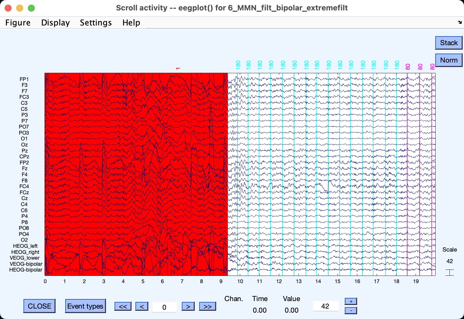
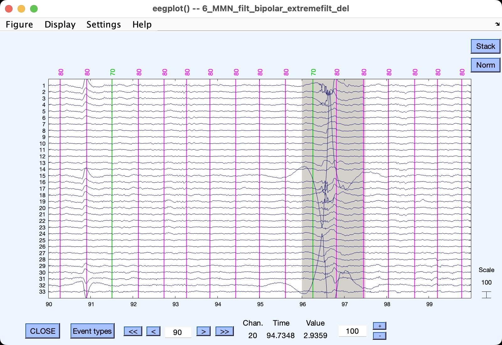
Make sure that the panel is set as shown in the screenshot, and then click Preview. You will see a window like the one shown in the screenshot below. Time periods that will be deleted are shaded in red. You can see that the first ~9 seconds are marked for deletion, with the deletion period ending 500 ms before the event code after the break. If you go to the end of the dataset (by typing 583 in the box between the < and > symbols), you can see that the break at the end of the dataset is also marked for deletion, with the deletion period starting 1500 ms after the last event code.
Now close the preview window, click Finalize in the Delete Time Segments panel, and save the new EEGset as 6_MMN_filt_bipolar_extremefilt_del. You can see that there is now a boundary event (code -99) at the beginning of the dataset, with the first real event (code 180) occurring 500 ms after the start of the EEGset.
Our last optimization step is to delete any remaining periods of large idiosyncratic artifacts. Remember, the goal is to get rid of large artifacts that do not have a consistent scalp distribution, not to get rid of the ordinary artifacts that ICA is meant to handle, such as blinks.
To accomplish this, go to the Reject Artifactual Time Segments panel. The best way to find large idiosyncratic artifacts is with a moving-window peak-to-peak algorithm. It divides the data into a set of short windows (e.g., 1000 ms long), and finds the difference between the minimum and maximum peaks in each of these windows. If this peak-to-peak voltage exceeds a criterion (e.g., 200 µV), that window will be deleted from the EEGset. Note that, unlike ERPLAB’s procedure for detecting artifacts in epoched EEG, which simply marks epochs that contain artifacts, the Reject Artifactual Time Segments panel actually deletes the artifactual segments from the EEGset.
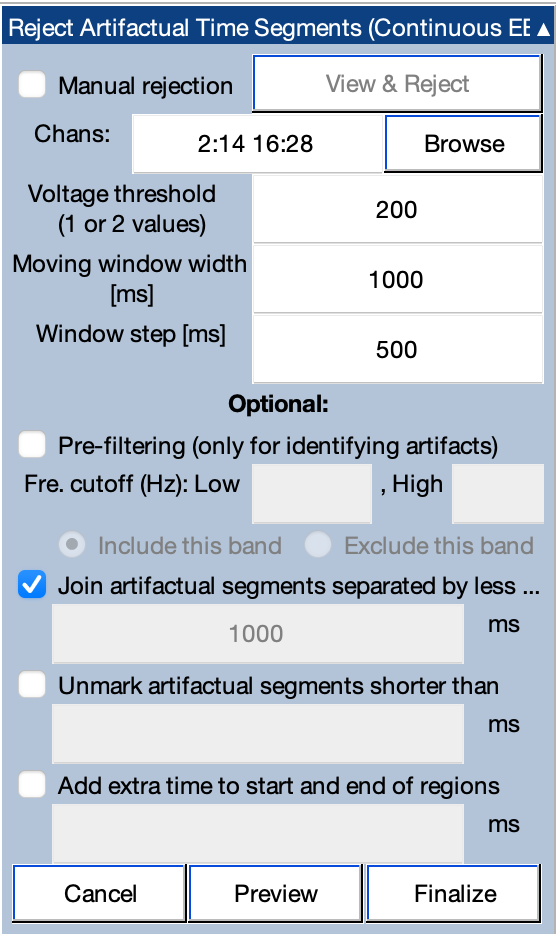
We don’t want to delete time periods that have large peak-to-peak amplitudes solely because of blinks, so we will exclude the channels with large blink activity from this procedure. To accomplish this, go to the Chans line in the Reject Artifactual Time Segments panel and click Browse. A window will appear that allows you to select which channels should be scanned for artifacts. Select all of the channels except FP1, FP2, and the VEOG and HEOG channels. The result should be 2:14 16:28 (as shown in the screenshot).
For this EEGset, a threshold of 200 µV will work well for identifying periods with large idiosyncratic artifacts, so enter 200 for the Voltage threshold. The appropriate threshold varies across datasets, so you may need to try a few different thresholds for your own data.
You can set 1000 for the moving window width and 500 for the window step. This will give you a set of 1000-ms windows that start every 500 ms. You should set Join artifactual segments to 1000. This will cause brief periods of unrejected data to become rejected.
Once you have set everything as shown in the screenshot, click Preview to see which data periods will be deleted. If you scroll through the data, you will see periods marked for deletion at approximately 96, 253, 402, and 413 seconds. These periods contain large and unusual artifacts that will degrade the ICA decomposition process. To actually delete them, you should close the preview window and click Finalize in the Reject Artifactual Time Segments panel. You should name the new EEGset 6_MMN_filt_bipolar_extremefilt_del_car and save it to disk as 6_MMN_filt_bipolar_extremefilt_del_car.set.
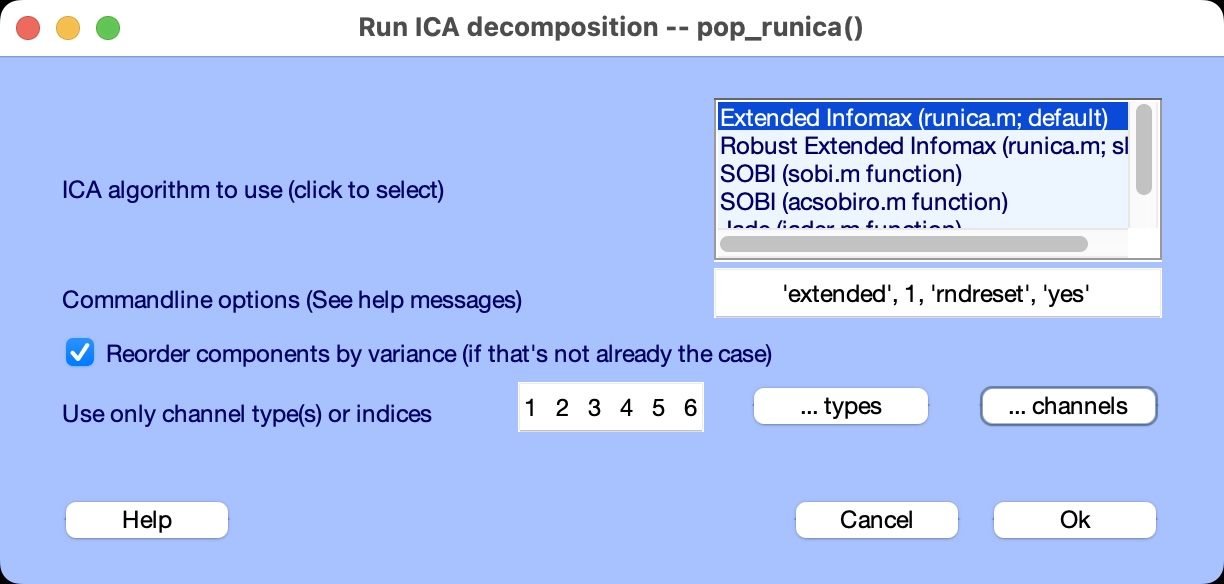
We are now ready to perform the ICA decomposition (i.e., compute the ICs for this EEGset). Make sure that 6_MMN_filt_bipolar_extremefilt_del_car is selected in the EEGsets panel, go to the EEGLAB ICA panel, and click Decompose data. You will see a window like the one in the screenshot below. Click the …channels button and select all of the channels except VEOG-bipolar and HEOG-bipolar (and click Ok). This will cause the ICA decomposition to ignore those channels.
Now click Ok in the ICA decomposition window to start the process. This process can take quite a bit of time (a few minutes). If you go to the Matlab Command Window, you can monitor its progress. When it is done, you should name the new EEGset 6_MMN_filt_bipolar_extremefilt_del_car_ica and save it to disk as 6_MMN_filt_bipolar_extremefilt_del_car_ica.set.
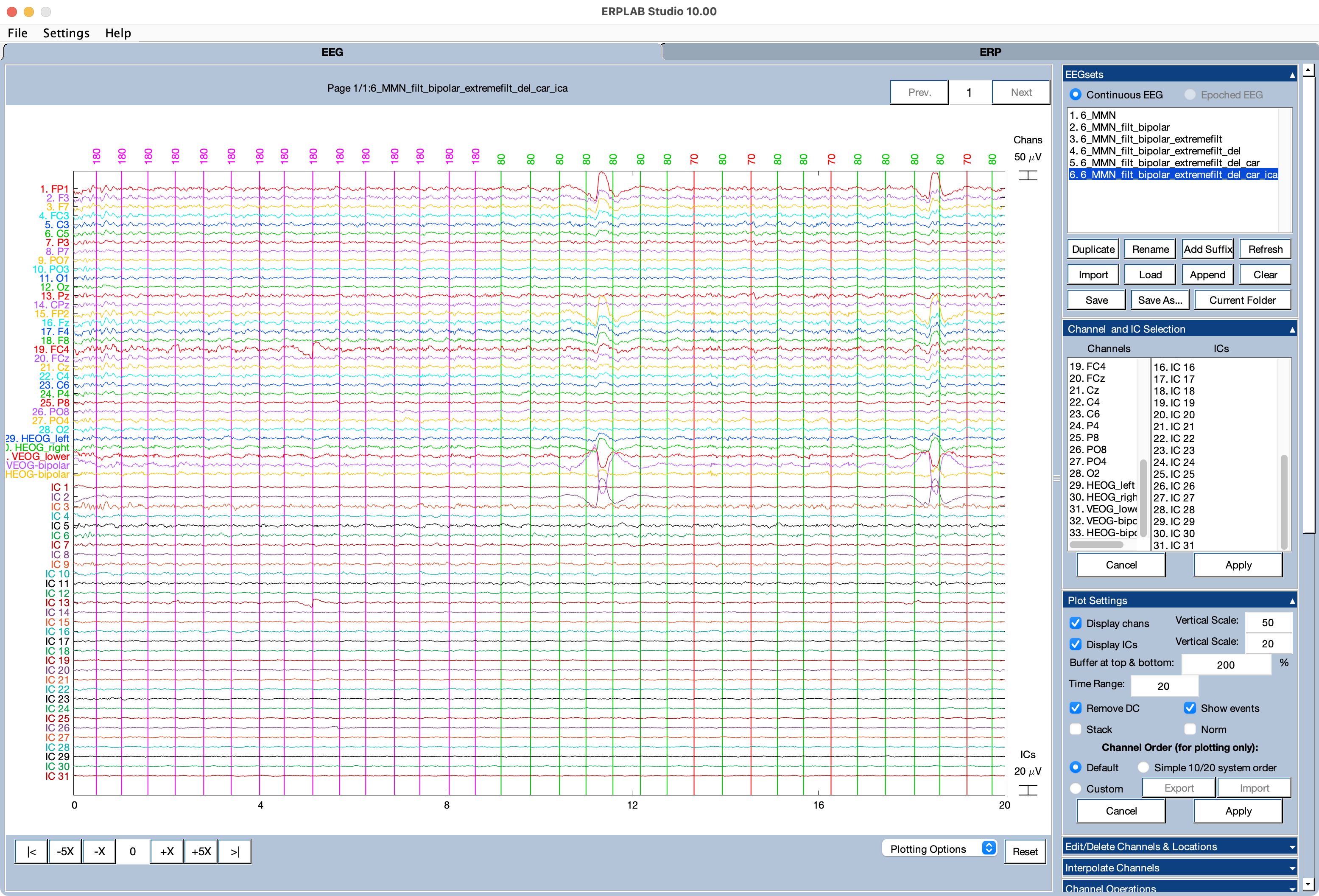
If you go to the Channel and IC Selection panel, you can see that there are now 31 ICs in your EEGset.
Go to the Plot Settings panel and check the box for Display ICs. This will cause the activation values to be shown in the plot region along with the voltages from the channels (see screenshot). You can see a clear blink just before 12 seconds in the EEG/EOG data, and a corresponding deflection in IC 2.
The ICA decomposition process involves training a machine learning algorithm to find the maximally independent components. The training starts with random weights, so the results may be a little different each time you run it on a given dataset. Don’t be concerned if the results you get in this tutorial look slightly different from what is shown in the screenshots. In some cases, the polarity of an IC may reverse, but that is not a problem.
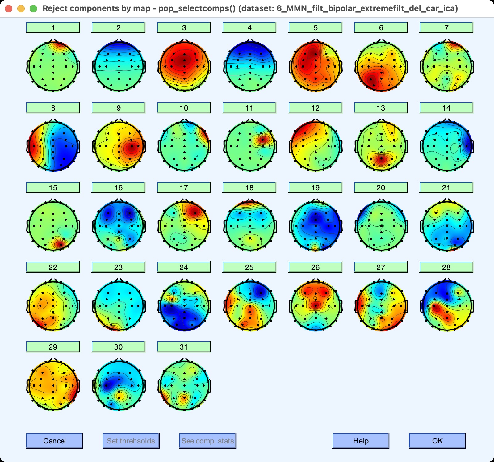
To see scalp maps of the ICs, go to the EEGLAB ICA panel and click Inspect/Label ICs. Tell it to plot all 31 components. You will then see a window like the one in the screenshot below. Note that IC 2 has the scalp distribution you would expect for blinks. You can’t use the scalp map alone to determine that an IC is a blink, but the match between the time course of IC 2 and its scalp map make it clear that it reflects blinking.
While the Inspect/Label ICs tool is running, the main ERPLAB Studio window will be frozen.
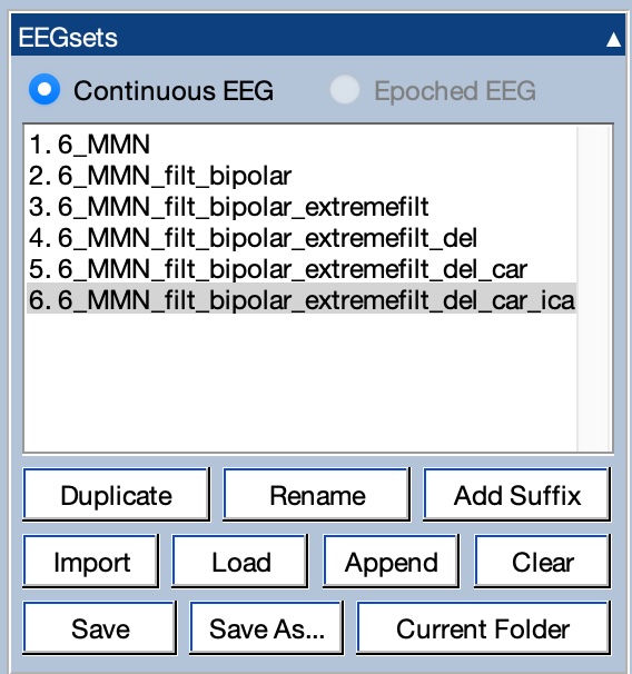
Now that we’ve done the ICA decomposition, it’s time to transfer the ICA weights back to the original dataset, 6_MMN_filt_bipolar. Make sure that this dataset is still available in the EEGsets panel and note the number of this dataset. For example, in the EEGsets panel shown in the screenshot here, 6_MMN_filt_bipolar is EEGset #2.
Now make sure that the dataset with the ICA weights is still selected (6_MMN_filt_bipolar_extremefilt_del_car_ica) and note the number of this dataset. In the EEGsets panel shown in the screenshot below, 6_MMN_filt_bipolar_extremefilt_del_car_ica is EEGset #6.
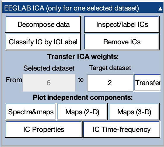
Look in the Transfer ICA weights section of the EEGLAB ICA panel, and you will see that the dataset number corresponding to 6_MMN_filt_bipolar_extremefilt_del_car_ica is set as the From dataset. Type the dataset number corresponding to 6_MMN_filt_bipolar in the box for the Target dataset, and click Transfer to transfer the weights from 6_MMN_filt_bipolar_extremefilt_del_car_ica to 6_MMN_filt_bipolar. Name the new EEGset 6_MMN_filt_bipolar_icaweights.
If you look at this EEGset, you will see that it contains the break periods with the large voltage swings along with large idiosyncratic artifacts at various points (e.g., around 105 seconds). The noise in the break periods isn’t a problem, because those periods won’t be in the EEG epochs used for averaging. And we will mark epochs with large artifacts when we perform artifact detection on the epoched data (and then exclude those epochs during averaging). Moreover, when we count the number of artifacts that were excluded because of averaging (which should be reported in published papers), those epochs will be included in the count.
Make sure Display ICs is active in the Plot Settings panel. If you scroll through the data, you will again see that IC #2 exhibits a voltage deflection at the time of each blink. This is the IC that we want to remove to eliminate the blink artifacts. (Note that this participant did not have many eye movements, so there is no clear IC corresponding to the eye movements in the HEOG channel.)
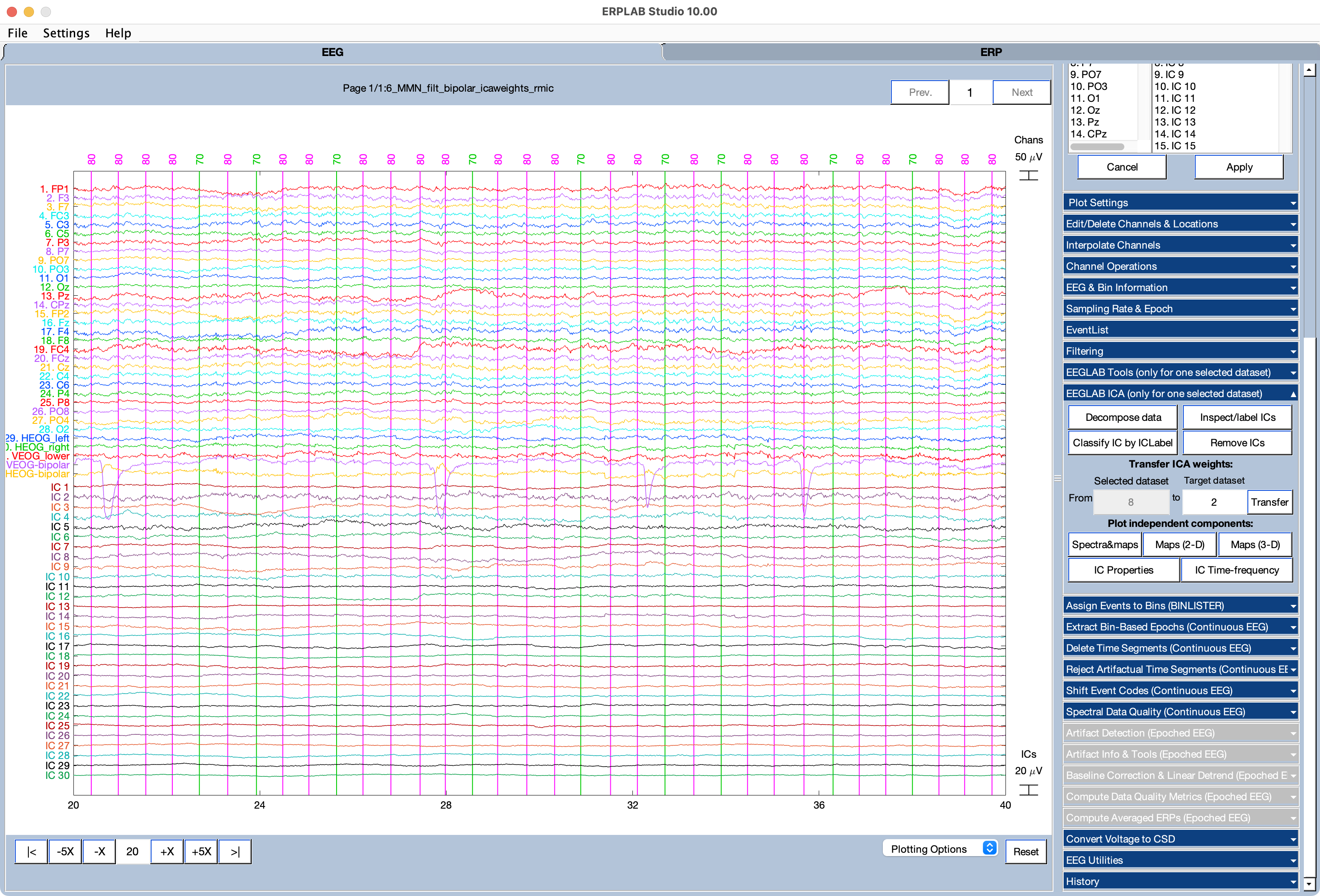
To remove the blinks from the EEG data, go to the EEGLAB ICA panel and click Remove ICs. Enter 2 in the text box labeled List of component(s) to remove from data in the window that appears, and then click Ok. Name the new EEGset 6_MMN_filt_bipolar_icaweights_rmic and save it to disk. This is now your corrected dataset.
If you look at the data from 20-40 seconds, you can still see blinks in the VEOG-bipolar channel (because the VEOG-bipolar and HEOG-bipolar channels were excluded from ICA). But these large voltage deflections are no longer accompanied by deflections in the FP1, FP2, and VEOG_lower channels. It worked!
| Previous Page | Next Page | 🏠 |
|---|---|---|
|
Interpolation |
Home |