Studio Tutorial: Filtering ERPs - ucdavis/erplab GitHub Wiki
Our next step will be to filter the ERPs. Filtering can be applied to continuous EEG data, epoched EEG data, or averaged ERPs. To avoid “edge artifacts”, high-pass filters should typically be applied only to continuous EEG data. However, low-pass filters can be applied at any stage. For an overview of the principles for determining the best order of processing steps, see the Appendix in An Introduction to the Event-Related Potential Technique (or click here for a summary).
If you don’t still have everything set up from the previous step of the tutorial, make sure that you have the ERPsets from all six participants (6_N400, 1_N400, 7_N400, 12_N400, 15_N400, 16_N400) and the grand average ERPset (named grand) in the ERPsets panel. You should also have the Grid Layout in the Plot Settings panel set to Custom using the file named GridLocations_Custom.tsv. The Show standard error option should be turned on in the Plot Settings panel, and bins 3-5 should be selected in the Bin & Channel Selection panel. It should look the screenshot below.

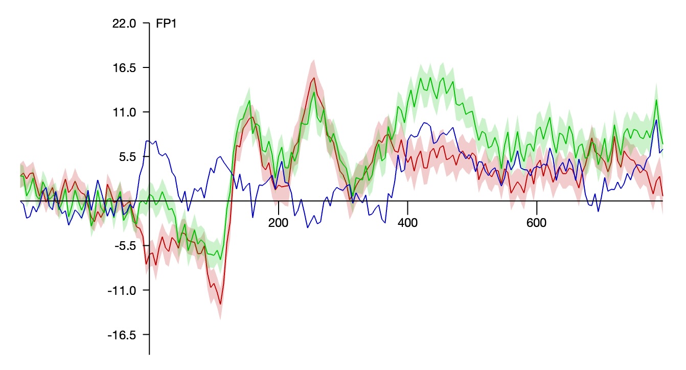
If you look at the ERP waveforms for the individual participants, you’ll see that some of them have a lot of high-frequency “fuzz”. A good example is the FP1 site from 16_N400, as shown in the screenshot below.

Now select grand in the ERPsets panel, go to the Filtering panel, and set it to apply a low-pass filter with a cutoff at 20 Hz and a roll-off of 12 dB/octave, as shown in the screenshot below. Click Run and name the new ERPset grand_filt. As shown in the screenshot, the ERP waveforms are now smoother than they were before.

However, the standard error is no longer plotted. This is because the original standard error values are no longer valid for the filtered data, so they have been removed. To get the standard error for the filtered waveforms, we will use the same trick we used to get the standard error for the difference wave, namely applying the processing operation to the single-participant ERPsets prior to making the grand average.
To do this, first select grand and grand_filt in the ERPsets panel and click Clear to clear these grand averages from memory. Now select the six single-participant ERPsets, go back to the Filtering panel, and click Run to apply the 20 Hz low-pass filter to the ERPsets. You’ll then see the window for saving the new ERPsets, and you should click Okay to confirm the names of the new ERPsets (which are the original names with _filt appended). You should now be able to see the six filtered ERPsets in the ERPsets panel.
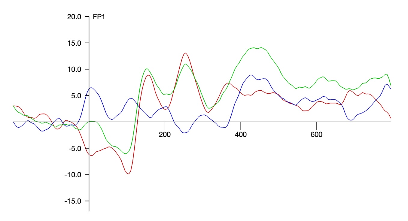
If you look at the FP1 site from 16_N400_filt, you’ll see that the high-frequency “fuzz” has been reduced.

Now we will make a grand average. With the six filtered ERPsets selected, go to the Average Across ERPsets panel (which should be set as shown in the previous steps), click Run to create the grand average, name it grand_filt, and save it to disk as grand_filt.erp.
If you go to Plot Settings and turn on the option to Show standard error (and click Apply), you should now see the filtered data along with the standard error shading (see screenshot below).

Note that SME values will not be present for any of the bins in the new grand average (or in the single-participant ERPsets). This is because the data quality is unknown for the filtered data. To obtain SME values for the filtered data, you would need to either apply the filter before averaging or use bootstrapping to compute the SME values from the filtered ERPs.
| Previous Page | Next Page | 🏠 |
|---|---|---|
|
Averaging (Channels) |
Home |