Prev (General Actions) | Home | Manual | Index | (Tips & tricks for online maps) Next

---

Table of contents

• Details of map use
  • Adjustable map properties
  • Use of map visibility range
  • Adjustable elevation properties
    • Range of use of elevation data
    • Hillshading
    • Slope shading
    • Slope coloring
    • Elevation limit
    • Elevation shading
  • Map scale type
  • Projection and datum
  • Fullscreen display
  • Distance ruler
  • Synchronization of map views

---

Details of map use

For basic information about this topic compare also the Control of Maps and DEM Files page!

Adjustable map properties

(valid starting with QMS patch version de4deeb (30.07.2017))

After activating a map in a map view, some properties that control the display of the map can be adjusted. The number of properties depends on the type of the map. Their availability is shown in the next table:

Property	vector map	offline raster map	online map
Map opacity	✔	✔	✔
Visibility range of map	✔	✔	✔
Visibility of object types	✔	✘	✘
Visibility of details	✔	✘	✘
Layout of map objects	✔	✘	✘
Cache size	✘	✘	✔
Cache expiration	✘	✘	✔
Layer selection	✘	✘	✔
Data opacity	✔	✔	✔
Fullscreen display	✔	✔	✔

The following image shows the layout of the various selection possibilities in the map tab:

Comments:

• Each map view has its own set of activated maps.
• Re-order the activated maps with drag-and-drop.c
• The map opacity slider controls the map visibility in a map overlay. Having several activated maps you can use this slider to look through a map to see the next one.
• The visibility range controls the zoom levels for which the map is displayed.
• The visibility of object types allows suppressing the display of some object types in the map.
• The visibility of details controls how many map details are shown at a given zoom level.
• The layout of map objects can be changed by using different type files for the map.
• The data opacity (slider in the data and not in the map tab!) controls the opacity of the GIS data in the workspace.
• Fullscreen display of a map window is enabled by pressing F11 (toggle!).

Use of map visibility range

A map visibility range is the range between some maximum zoom level and some minimum zoom level at which the map is visible in a QMS map view.

Vector and raster maps loaded into QMS have, in general, 2 visibility ranges:

• A predefined visibility range defined with the map itself.
• A user-controlled visibility range.

The user-defined visibility range of a map is controlled with the help of the visibility range slider in the docked map window. To define such a range proceed as follows:

• Check if the buttons on the left and the right side of the slider are both green. If not, then click on each red button to change its color to green. If both bottoms are green, then the map is displayed on all zoom levels.
• Zoom in the map up to the wanted maximum zoom.
• Click the small icon on the left side of the slider. The button changes its color to red as an indication that a range limit is defined.
• Zoom out the map up to the wanted minimum zoom.
• Click the small icon on the right side of the slider. The button changes its color to red as an indication that a range limit is defined.

A green line segment in the visibility slider now shows the user-defined visibility range for the map. When zooming the map, a slider handle moves along the slider. As soon as it is in the green range, the map is visible.

To change a visibility range click the button on the side of the range you want to change. The button color changes to green. Select the new zoom level and click again the same button to define a new size of the range.

A visibility range can be removed by clicking on the red buttons on the left and the right side of the slider.

This feature allows you to switch from one map to another one depending on the zoom level. Simply activate the maps to be used and define for the maps consecutive visibility ranges as shown in the following images.

If visibility ranges of activated maps overlap, then the lowest activated map in the maps list is drawn.

In the following example, 4 different maps of different types with different levels of detail are activated. Each map has its visibility range. The ranges are disjoint. The waypoint on the map (red diamond near the lower right corner) is shown on 4 different maps depending on the zoom level (check the slider handle positions). The details in the map decrease when decreasing the scale of the map (when zooming out).

Adjustable elevation properties

(valid starting with pull request [QMS-487], commit 1371478, Fri Feb 18 01:57:31 2022 +0100)

After activating elevation data (DEM data), some properties that control the rendering of this data in a map view can be adjusted.

The following image shows the layout of the various selection and rendering possibilities in the DEM window for an activated DEM data set:

List of properties (from top to bottom):

• Filter field to find your DEM data set in the list of loaded DEM data sets (type the name of the DEM data into the edit field)
• Name of DEM data set. A small triangle in front of the name indicates that the DEM data is active, i.e. used by QMS. Clicking the triangle opens the adjustable properties for this DEM data set:
  • Opacity of all DEM data related map overlays
  • Visibility range (zoom range where DEM data is used)
  • Hillshading with intensity slider
  • Slope shading (grayscale shading) with intensity slider
  • Slope coloring
  • Ranges used for slope coloring with predefined and custom slope settings
  • Elevation limit
  • Elevation shading (show elevation by color)
  • Minimum and maximum elevation used for elevation shading

Comments:

• The opacity slider controls the visibility (opacity) of the hillshading, slope, elevation limit, and elevation shading layers on a map.
• The visibility range controls the zoom levels for which hillshading, slope, elevation limit, and elevation shading layers are displayed.
• The hillshading slider controls the intensity used for the display of hillshading.
• The slope selection allows choosing one of the predefined slope models. In the case of the "custom" model, the user can define 5 personal slope levels (click on a value and adjust it).
• If the elevation limit property is selected, then an extra magenta-colored layer is drawn on the map showing areas above the given limit. This is of special interest when planning aviation routes.
• Tooltips are available for the slider and the label fields.
• All elevation-related properties work best if high-precision DEM data sets are used.
• DEM data sets consist of single tiles. From time to time these tiles don't fit together smoothly. One reason for this can be a necessary preliminary format and coordinate system transformation step to make the data accessible for QMS. This explains the small strips in the following images.

Range of use of elevation data

A range of use of elevation data is the range between some maximum zoom level and some minimum zoom level at which the DEM data is used in a QMS map view for creating data objects, for hillshading, for showing slopes, and for some other purposes.

Elevation data can be considered as some kind of map (an elevation map). That is the reason why elevation range selection is done in the same way as for visibility range selection of maps. Therefore, the handling of the range selection slider is not repeated here.

DEM files may consist of data with different precision. Defining (disjoint) use ranges for each DEM file makes it possible to use high precision elevation data when zoomed to a level with high detail of the map and to use less precise elevation data when working with an overview map.

The magenta overlay in the next image shows the area where elevation data of the used DEM file N51E010 is available. Here, a use range is not selected (both slider buttons are green). The QMS status line displays the elevation at the mouse pointer if it is inside the data range of this DEM file. Elevation data from this DEM file is not available for locations outside the magenta area.

Now, let's activate a second DEM file, and let's define a use range for each of the files:

The zoom in the left image is in the use range of the first DEM file (check the position of the slider handle!) but not in the use range of the second DEM file. In this situation, the slope is activated and shown because elevation data is available at this zoom level from the first DEM file. A magenta elevation limit overlay is not displayed. It is only active for the second DEM file. Elevation data for this DEM file is not available at the given zoom level.

The zoom level in the right image is in the use range of the second DEM file but not in the use range of the first DEM file. Here, the magenta elevation limit is active and shown. Slopes are not shown. They are not active for the second DEM file. Elevation data is not available at this zoom level for the first DEM file.

This example demonstrates how slope, hillshading, and other elevation features can be made dependent on the zoom level.

If use ranges of activated DEM files overlap, then all elevation-dependent features of all DEM files in the intersection of the use ranges are displayed as shown in the next image. Here, the slope is derived from the first DEM file and the elevation limit (the magenta-colored part around the waypoint at the summit) from the second one. The magenta area is opaque due to the opacity setting for the second DEM file. Thus, in this area, the slope below the magenta area is visible, too.

If no ranges are defined, then all features selected in all DEM files are drawn as well.

If elevation data is required for a data object, the activated DEM files are searched starting with the top-most one for valid elevation data. Elevation data is taken from the first DEM file that can provide it regardless of the use ranges. As a consequence, activated DEM files should be arranged by the precision of the elevation data with the highest precision on top.

The behavior of the elevation-related data under the mouse cursor (the ones shown in the status line of the QMS GUI) is slightly different. In this case, the use ranges are respected. Elevation and slope at the mouse cursor are taken from the first DEM file with a matching use range containing the elevation for the given position. If there is no matching range, then elevation is not shown in the status bar.

Hillshading

Hillshading simulates a 3-dimensional terrain view based on DEM data by shading light from the northwest on the terrain. Hillshading is activated with a click on the hillshading checkbox. The hillshading slider controls the intensity of hillshading (moving the slider to the right decreases the intensity):

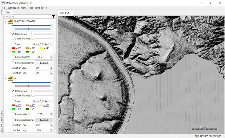
The gray area in the lower right part of the previous image is a result of missing DEM data in this area.

The next image demonstrates the importance of the quality of DEM data for hillshading. The previous image belongs to DEM data with a 1 m grid while the following image belongs to DEM data with a much coarser grid. The result is a more or less washed-out image.

Several DEM data sets can be used at the same time as shown in the next image. Here, low-quality DEM data is used in the lower right part of the image and high-quality data in the rest of the image. The opacity of the high precision layer ("lsn" data set) was reduced (check opacity slider position!) so that the lower quality layer can be seen, too.

Using the opacity slider the hillshading layer can be combined with the underlying map layer as can be seen in the next image.

Slope shading

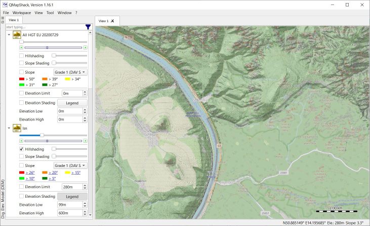
Slope shading shows the steepness of a terrain. Slope shading is activated with a click on the slope shading checkbox. The slope shading slider controls the intensity of slope shading (moving the slider to the right increases the intensity). The next image shows how slope shading works in combination with an underlying map:

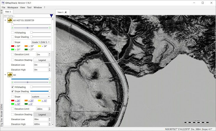
Slope and hillshading can be combined (in the next image the underlying map is not shown):

Using the opacity slider the underlying map can be revealed, too:

Zooming-in gives a good 3-dimensional impression of the terrain together with the map:

Slope coloring

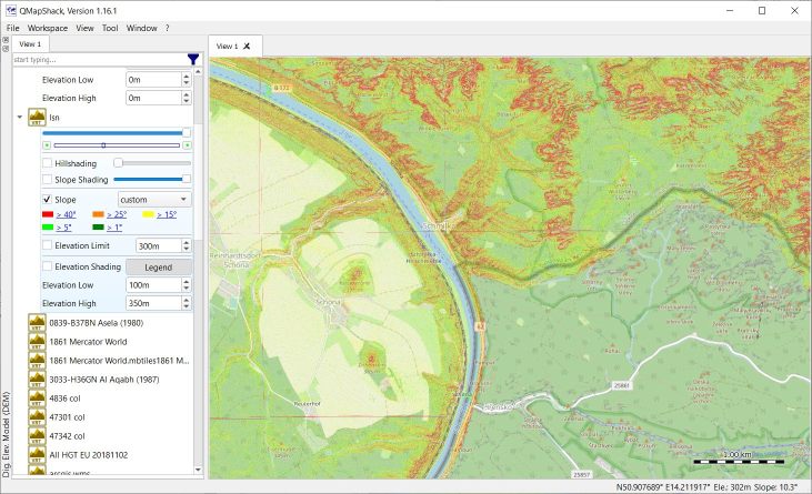
Clicking the slope checkbox predefined or user-defined (custom) slope ranges are mapped to different colors. The colors are then shown as an overlay on the base map. The combobox can be used to select between several predefined or customized settings. In the case of custom settings, click a setting and change its value.

Elevation limit

Clicking the elevation limit checkbox and setting an elevation limit in the spinbox creates a magenta layer showing all parts of the terrain with an elevation above the selected limit:

Elevation shading

(implemented with pull request QM-476, 2022-01-24 13:57 MEZ)

This feature is using a color spectrum to show elevation. To do this click the elevation shading checkbox and set values for the lower and the upper limits for the color spectrum. Press the Legend button (gray button background if pressed) to show a legend at the top-right edge of the map window. Use the opacity slider for changing the visibility of the background map.

The precision of the coloring depends on the precision of the DEM data used. In the following snapshot, a worldwide and therefore less precise data model is used for almost the same area as above to show the difference.

The next snapshot was created with the help of a DEM data set with a 1 m grid size. Gray areas either don't have elevation data (dark gray) or elevation data not in the selected elevation intervall (light gray).

Combing elevation, slope, hillshading, and a map results in the following realistic image of the terrain:

Map scale type

Selecting the menu View - Setup Map View opens a map view setup window. In this window, the user can set the map scales to Logarithmic or Square.

A change of this option leads to a different zoom behavior of maps.

Logarithmic scales support more zoom levels than square ones. As a consequence, zooming with a square scale changes the scale faster than zooming with a logarithmic scale.

The minimum and maximum zoom levels (scales) are nearly the same for both scales.

For square scales, the next zoom step leads to a scale that is approximately changed by a factor of 2 compared with the previous one. This scale is recommended for online (TMS, WMTS) maps.

Projection and datum

The projection and geodetic datum (in short: the coordinate systems) for map rendering and grid display can be defined separately for each view. To do this, use the menu entries View - Setup map view and View - Setup grid.

Recommended (default) settings are:

• for map rendering: projection: Mercator, datum: WGS_1984, used setup string (Proj.4 format):

    +proj=merc +a=6378137.0000 +b=6356752.3142 +towgs84=0,0,0,0,0,0,0 +units=m +no_defs
  

• for grid display: projection: lon/lat (geographical coordinates), datum: WGS_1984, used setup string (Proj.4 format):

    +proj=longlat +datum=WGS84 +no_defs
  

These settings use the format of the Proj.4 project. For details see the project documentation which can be downloaded from here.

Remark: For map rendering projections using lat/lon coordinates are not supported. Don't use Proj.4 settings with +proj=longlat!

The status line at the bottom of the QMS window shows always the geographical coordinates of the mouse location on the map. The map is rendered so that the edges of the map view have constant first resp. second coordinate as defined with the coordinate system for the map.

If the grid display is switched on (use menu entry View - Show grid), then gridlines are drawn on the map. In general, gridlines are curves connecting points on the map with equal first resp. second coordinate (in the default case: latitude resp. longitude). Grid coordinates are shown in the status line within square brackets after the geographical coordinates.

If the map coordinate system and the grid coordinate system are equal, then the gridlines are straight lines parallel to the edges of the map view.

Some properties of coordinate systems are illustrated in the following images using a map for the whole of Germany:

• Map and grid settings as mentioned at the beginning of this section:

  • default WGS84 display of map and grid
  • coordinates are longitude and latitude
  • map and grid coordinates are equal
  • straight gridline
  • gridlines parallel to the edges of the map view
  • coordinates and grid coordinates in the status line are equal
  • grid coordinates displayed at the edges of the map view show longitude and latitude

  

• Map setting changed to UTM, zone 32, grid settings unchanged:

  • new map setting:

      +proj=utm +zone=32  +a=6378137.0000 +b=6356752.3142 +towgs84=0,0,0,0,0,0,0 +units=m  +no_defs
    

  • grid coordinates are still longitude and latitude

  • map coordinates are UTM (northing/easting)

  • as a consequence of UTM coordinates in the map and lon/lat coordinates in the grid: gridlines are curved

  • edges of the map view have constant northing resp. easting values

  • map is distorted compared with the previous image due to the use of different coordinate systems

  • coordinates and grid coordinates in the status line are equal (even if the coordinates used for map rendering have changed, the location on the map is always shown with lat/lon coordinates)

  • grid coordinates at the edges of the map window show longitude and latitude

  

• Map setting changed to UTM, zone 32, grid changed to UTM, zone 32:

  • new grid setting:

      +proj=utm +zone=32  +a=6378137.0000 +b=6356752.3142 +towgs84=0,0,0,0,0,0,0 +units=m  +no_defs
    

  • grid coordinates are UTM (northing/easting)

  • map coordinates are UTM (northing/easting) and equal to grid coordinates

  • edges of the map view have constant northing resp. easting (latitude resp. longitude vary along these edges!)

  • carefully comparing the next image with the first one in this section shows that there is again a distortion due to the use of different coordinate systems in the 2 images.

  • straight gridlines

  • gridlines parallel to the edges of the map view

  • grid coordinates at the edges of the map window show northing resp. easting

  • coordinates in the status line are different: lon/lat followed by UTM for grid

  

Remarks:

• Curved gridlines and map distortion are clearly visible if the map is displayed at a large scale. The smaller the map area displayed in the map view the less obvious are these distortions.

• A side effect of using coordinate systems with different features is the change of the map scale when moving the map over long distances to the north or south (not zooming the map).

• Many projections are defined for use within a certain region (e.g. a UTM zone). Using such a projection outside its area of definition (e.g. in a different UTM zone) may lead to weird screen results.

• Often geographical lon/lat coordinates are given without mentioning the used coordinate system. A typical situation is the use of some national coordinate system. The following image shows map and grid coordinates in lon/lat format. The map coordinate system is the international WGS84 one, the grid coordinate system is the German Potsdam datum. WPT2 is located at 50° North (WGS84/map coordinate), the corresponding grid coordinate is 50.001162° North (Potsdam datum). WPT1 is a WPT located at 50° North (Potsdam datum). The distance between both waypoints is more than 100 m. This demonstrates also the danger of using coordinates with an unknown coordinate system (can happen with coordinates from printed raster maps). Trying different grid settings can help to identify the coordinate system which was used when describing a waypoint.

  

Fullscreen display

(valid starting with QMS patch version de4deeb (30.07.2017))

Map windows (and other windows as well) can be displayed in fullscreen mode. A map window switches to fullscreen mode after pressing F11. Pressing F11 again switches the window back to the standard mode.

Remarks:

• If the QMS toolbar is active, then it is also shown in the fullscreen window.
• Pressing CTRL-D in the fullscreen mode activates the docked windows. Pressing this key again closes the docked windows in the fullscreen mode.

Distance ruler

(valid starting with QMS patch version bf60cdce289a (13.08.2018))

The purpose of the distance ruler is to find distances along straight line segments in a map view window.

To use the distance rule proceed as follows:

• Open a map view.

• Right-click with the mouse in the map view to open the context menu and select the menu entry Ruler. The mouse icon will change to the ruler icon . A ruler toolbar pops up at the upper left corner of the map view. Bubble boxes explain the meaning of each toolbar icon when moving the mouse on it. The icons in the middle of the toolbar have 2 states: "pressed/selected" or "not pressed/selected".

  

  The following table gives an overview of the toolbar:

Default icon	Tooltip
	Convert into a group of waypoints.
	Convert into a track.
	Convert into a route.
	Convert into an area.
	Show table.
	Show course of each segment.
	Show ascent or descent of each segment.
	Show angle between line segments.
	Show distances in high precision.
	Reset ruler.
	Undo
	Redo

• Left-click in the map view at the first point of the wanted line segment.

• Add points with more left-clicks.

• Right-click, if finished with adding points (line segments).

• Assume all selectable toolbar icons are selected. Then a table shows information about the length (distance) and other information of each line segment. The same information is displayed on the line segments. In addition to this, the angle between adjacent line segments is shown.

  

• Using the respective toolbar icon, the ruler line segments can be converted into a track, a route, or an area. The endpoints of the line segments can be converted into waypoints.

• Hints:

  • If the supplied waypoint name ends with a digit, then the waypoints are numbered consecutively as shown in the next image. Otherwise, all waypoints get the same name.

    

  • Tracks generated in this way consist simply of straight line segments.

  • Routes generated in this way can be recalculated using a routing engine (select menu entry Calculate route from the route context menu).

    

  • The 2 comboboxes in the ruler toolbar can be used to select a fixed distance and a fixed angle. In this case, the segments have lengths that are multiples of the given distance and the angles between segments are multiples of the given angle.

    

• Finally, press the Close button in the toolbar to close the ruler tool.

Synchronization of map views

Feature available starting with QMS dev version commit b423c02 (May 8 11:31:02 2021 +0200)!

QMS can display maps in one or several map views. As an example, assume that one map view displays a road map, another one orthophotos for the region shown on the road map.

When moving or zooming the map in one view it can be desirable that the maps in the other views perform the same operation so that maps in different views remain in sync.

This synchronization of maps in different map views can be switched on with the menu entry View - Link map views. Selecting this menu entry again switches off the synchronization.

Remark: Maps in different map views may use different projection and datum and scales. As a result of this, a rectangular map area in one view may fail to be a rectangular area in the other view. Synchronization is not possible in such a case. Thus, before using map synchronization the user has to ensure equal map projections, datums, and scales in the map views. Otherwise, the following error message is shown and synchronization is switched off:

---

Prev (General Actions) | Home | Manual | Index | Top | (Tips & tricks for online maps) Next