Lekan allows delineating automatically watershed from a raster DEM.

First, if there is no DEM registered, it is necessary to register the raster layer as a DEM: right-click on the layer and choose "Register as Digital Elevation Model". Severals raster layer can be registered as a DEM, and an indicator is present to inform the user the layer is registered as a DEM ().

Then open the "Watershed Delineating Tool" . Note than the user can also load the raster DEM layer in the delineate tool window with the button on the right of the DEM selection combo box.

Be sure to be in the "Automatic from DEM" mode and choose the DEM wanted.

The check box "Calculate average elevation" allow the user to enable/disable this calculation during delineating if he is not interested by this parameter. Indeed, this operation can slow down the delineating.

Then click on the "Draw downstream line" button . Here the aim is to draw the line that intersects the flow on the downstream extremity of the watershed. So, draw this line on the map. Right-click to finish the drawing.

If the first watershed delineated or the new delineating is outside any already delineated watershed, it is necessary to choose an estimated extent of the watershed. It is necessary to avoid the algorithm to consider all the raster DEM, which would take too much time.

If necessary, the map tool is automatically selected, so draw the rectangle on the map (keep press the left button and release once the extent is defined).

Then press the "Delineate Watershed" button (if everything is OK, this button is now enabled), and the watershed will be delineated.

If the delineating intersect the estimated extent, it will be necessary to define this extent again.

If not, the "Validate Watershed" button will be enabled. Press it to validate the watershed. Then the watershed tree will be populated with the new one.

To delineate other watersheds, repeat the process.

Note that if the downstream line is drawn in an existing automatically delineated watershed with the same raster DEM, the algorithm will use the previous calculation to delineate the new one, that why it is faster to delineate a subwatershed. There is no need to draw an estimated extent.

There is also the possibility to use burning lines . With these lines, the DEM level will be burnt on the line; that is to say, the level on each point will be interpolated between the level of the extremity of the burning line. This could be useful, for example, to go through road embankments, DEM imprecision or errors.

It is also possible to delineate watershed manually, drawing a polygon with the mouse.

Choose the mode "Manual delineating", then use the map tool "Draw watershed manually" on the same windows.

Draw the polygon of the watershed delineating and right-click when finished. As Lekan needs to know the watershed's outlet point, click where this outlet is to terminate the digitizing. Then validation of the watershed is possible in the delineating windows. This validation will send this new watershed to the watershed tree.

It is also possible to edit an existing watershed with the map tool "Edit watershed manually" . This edition is also possible for automatically delineated watersheds. The ediition allows:

• insert, remove or move vertices of the delineating polygon of the watershed
• move the outlet point of the watershed

The watershed tree is the place where the user can access watersheds and associated functionalities. Watersheds are organized in a watershed / sub-watershed hierarchy, that is, subwatersheds are children of containing watershed. This tree also includes the residual watersheds that are the remaining area next to subwatersheds.

Right-click on a watershed gives access to functionalities.

Watershed can also be selected from the map using the tool "Select watershed on the map" . Right-click also gives access to functionalities.

Just on the top of the tree, differents buttons allows the user to open specific windows:

• Longitudinal profile
• Concentration time
• Meteorological models
• Runoff hydrograph calculation
• Gauged hydrographs

On the bottom of the tree, the main characteristics of the watershed are displayed and can be changed. There is also a button to add/remove the watershed to/from the hydraulic network.

The window Longitudinal profile, opened with the button of the watershed tree, allows the user to work on the longitudinal profile of each watershed.

When delineating watershed automatically, the algorithm also defines the longest hydraulic path of the watershed. Here the user can edit this path with the following tools:

• Draw the flow path on the map, with the mouse
• Edit the flow path on the map, with the mouse (move, insert, remove vertices)
• Draw the longest path automatically from downstream (return to default state)
• Draw the longest path automatically from an upstream point chosen on the map

On this window's plot, the blue curve represents the current DEM projection on the flow path, which is the longitudinal profile defined by the current DEM.

Because there are too many points and this profile is often too irregular, the user has to define a theoretical longitudinal profile that will be used to estimate:

• the average slope of the watershed
• the length of the longest path
• the drop

These parameters are used to estimate the concentration time (see below).

The average slope is calculated with the following formula:

Where:

• L is the length of each segment
• p is the slope of each segment

The grey lines on the plot represent this theoretical profile. By default, ii is a simple line that links the extremity points of the DEM profile.

The tools available to defined the theoretical profile are:

• Draw the profile on the plot
• Edit the profile on the plot (move, insert, remove vertices)

It is also possible to edit or add vertices in the table on the right.

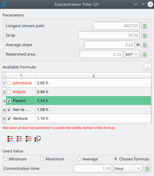
The window Concentration Time, opened with the button of the watershed tree, allows the user to calculate the concentration time of each watershed.

Important note: The parameters related to the longitudinal profile used to calculate the concentration will not be automatically calculated if the longitudinal profile window is not opened before. This a principle to "force" the user to check the longitudinal profile before this calculation. This principle is often applied in Lekan, also for the concentration time: if this window is not opened, the concentration time parameter will not be valid elsewhere. Lekan should not be a "black box"; the user has to know what is going on and control the process.

The user can override parameters on the top that are derived from the delineating and the longitudinal profile.

The tab contains all the available formulas (if you want more, fill an issue here ) with the calculated value. Red ones are the formulas for which at least one parameter is outside the formula's validity domain. The red formulas are unchecked by default, but the user can check them to consider them.

On the bottom, the user must choose how the concentration time is retained:

• minimum checked value
• maximum checked value
• average value from the checked value
• chosen formula, to select it, the user double-clicks on the formula in the table, the chosen one will have a green background

There are also convenient tools:

• Check all formulas
• Uncheck all formulas
• Check only valid formulas
• Copy to clipboard the checked results

A meteorological model is a set of associations between rainfall and watershed. To allow the user to organize his project with consistency, the meteorological model offers a way to group rainfall/watershed association. So, the meteorological model can be associated with a return period or a specific historical event.

Pushing the meteorological model button of the watershed tree will open the meteorological model window :

On the left, the rainfall tree is present with all the items (not editable). On the right, this is the watershed tree.

First, the user has to select the current meteorological model on the top. The following tools are provided to manage the available meteorological model :

• Add meteorological model
• Duplicate a meteorological model
• Remove the current meteorological model
• Rename the current meteorological model

Once the user has selected the current meteorological model, dragging a rainfall item with the mouse and drop it in the watershed is enough to associate a rainfall with a watershed. To remove this association, right-click on the watershed and choose "Disassociate rainfall".

Runoff manager is where the user can store runoff models. The runoff manager can be opened with the runoff manager button in the main toolbar.

All the runoff manager data are saved on the disk under a specific file that is still the same with any project. This allows keeping runoff model from one project to others. When opening Lekan (new project or with an existing project), the runoff manager load always the same file and this file is the last saved one. It is also possible to open another file, and then this one will be loaded by default for the next start of Lekan. But it is recommended to work with the same file to avoid bad reference to runoff models if the user changes the file during editing a project.

The runoff models supported are:

• constant coefficient: the same constant factor will always be applied to the rainfall. This coefficient must be between 0 and 1
• Green Ampt model, based on the Green-Ampt infiltration equation
• Curve Number model

A right-click on one of this group open a context menu where the user can add a new model or remove an existing one.

Runoff hydrographs calculations are handle in a specific window that is opened using the runoff hydrograph button of the watershed tree.

To generate a runoff hydrograph, the user has to choose a meteorological model that has been defined (see Meteorological models). This meteorological model is the way to associate rainfall with the watershed.

Some information about the corresponding rainfall is displayed under the meteorological model choice.

To associate a runoff model with the watershed, a right-click on the cell at the bottom of the runoff table ( and the first column) displays a context menu where the user can choose one of the runoff model available (see Runoff manager). Choosing a runoff model here will add it to the table.

To change the runoff model, a right-click on the first column of its row will display the context menu again to choose another one.

Each watershed can be associated with one or several runoff models, and for a specific watershed, the runoff is associated with a portion of the watershed area. The sum of each portion has to be 1.00. So, if there is only one runoff, the portion is always 1.00. With several runoff models, the watershed has to be shared between runoff models. If the portion of runoff is changed, the others' portions will be changed aromatically to have a sum of portion equal to 1.00. To help the user to set the portion for each runoff model, the user can lock a runoff model by checking the last column ( ).

The last step before obtaining the runoff hydrograph is to choose a transfer function, which is the method that will transform the runoff in a hydrograph.

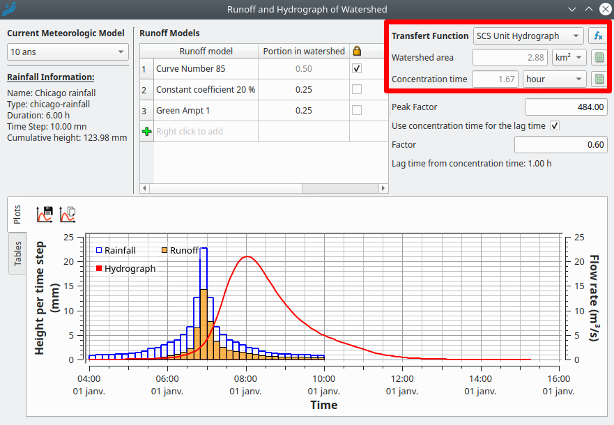
The available transfer functions are :

• linear reservoir
• Generalized Rational Method Unit Hydrograph
• SCS Unit Hydrograph

The Linear Reservoir Method is expressing the flow rate for the nth time step as below:

Where:

• Δt: the time step of the runoff
• t_l: the lag time
• A: the watershed area
• r: the runoff intensity or the effective rainfall intensity during the time step in mm per unit time
• Q₀ = 0

With Lekan, for the lag time, the user can choose to use the concentration time to calculate the lag time : a constant factor will be apply to obtain the lag time from the concentration time.

The Generalized Rational Method is a Unit Hydrograph transfer function. This Unit Hydrograph is defined as below:

Where:

• Δt: the time step of the runoff
• t_c: the concentration time
• A: the watershed area
• r: the runoff intensity or the effective rainfall intensity during the time step in mm per unit time

The SCS Unit Hydrograph defines a Unit Hydrograph with predefined hydrograph shapes depending on a peak factor. This peak factor links the peak flow rate and the peak time as below:

• Q_p: the peak flow rate for an effective rainfall height or a runoff of 1 cm
• T_p: the time of the peak in hours
• A: the watershed area in km2
• P_f: the peak factor between 100 and 600 with a typical value of 484. Peak factor with high value is for watershed with quick reaction (mountain), and lower values are for slower watersheds (plain).

With Lekan, the time of the peak is calculated from the lag time. For the lag time, the user can enter it directly or use the concentration time with a constant time factor.

Since version 2.2, Lekan allow the user to associate gauged hydrographs to watersheds. Then, these hydrographs can either be displayed with calculated runoff hydrograph for comparison or used as input hydrograph in the hydraulic network.

To add a gauged hydrograph, the user has two options:

• enter manually a new hydrograph after pressing the button
• Import a gauges hydrograph from a external sources using one of the data provider available (button(s) on the top left), see Delft-FEWS provider and Hubeau provider.

Editing a imported hydrograph is only possible if this hydrograph is imported as a copy or if the data provider of this hydrograph allow editing.

All gauged hydrograph can be removed or rename.