data pipeline - syue99/Lab_control GitHub Wiki

In this page we talk about what does the experimental data looks like (especially with camera) and how data flows in a real experiment.

Data Format for an experiment

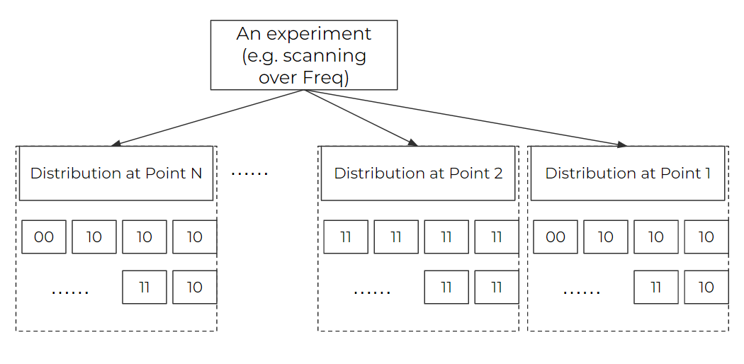
As in a quantum experiment, single shot is limited by the quantum projection noise, we have to repeat doing the same experiment to get a statistical distribution to get the actual quantum states. On the top of this statistical distribution, we often also need to repeat the experiment with different values of the independent variable (especially when scanning some parameter spaces). As the graph below shows, the data we have usually follow such a 2D structures. An experiment scanning M points will have M lists, for every list contains N repetition samples (can be different data like PMT/camera value, the graph below shows the 2 qubits' configuration as an example).

In an experiment, we care about 1. displaying the data (on the grapher), 2. saving the raw data. As a result, we handle our data to meet the two points above.

RAW Data

For the raw data, we just try to wrap up the 2D structure above. In fact, we keep a (2+L)-dim array (for L is the original data dim of every sample) and then save them into a .npy file at the directory of the experiment's data folder (under the datavault folder). For example, if we handle with the qubit configuration as a sample as the graph above shows, we will have a 2d array like [00,10,10,10,10,..,11,10],[11,11,11,11...,11],..[00,10,10,...,11,10](/syue99/Lab_control/wiki/00,10,10,10,10,..,11,10],[11,11,11,11...,11],..[00,10,10,...,11,10). If we use a single(two) channel PMT, the qubit configuration will be replaced by an integer (or list of two integers) of PMT readings. If we use camera, we will have a 4d array like [image1ofpoint1,image2ofpoint1,....,imageNofpoint1],[image1ofpoint2,...,imageNofpoint2],..,[image1ofpointM,...,imageNofpointM](/syue99/Lab_control/wiki/image1ofpoint1,image2ofpoint1,....,imageNofpoint1],[image1ofpoint2,...,imageNofpoint2],..,[image1ofpointM,...,imageNofpointM). Note as the raw data can be very big and we do not want to view them on grapher in real time, it does not go through the datavault. We save under the datavault's folder just for the sake of keeping all data of an experiment in the same folder.

Display Data

As the display data will go through the datavault, we usually need to do some pre-processing as the raw data is huge. Usually this is in the process of the data pipeline that we will discuss later. Depending on the different purposes of the experiment, we have three different types of display data

Linegraph

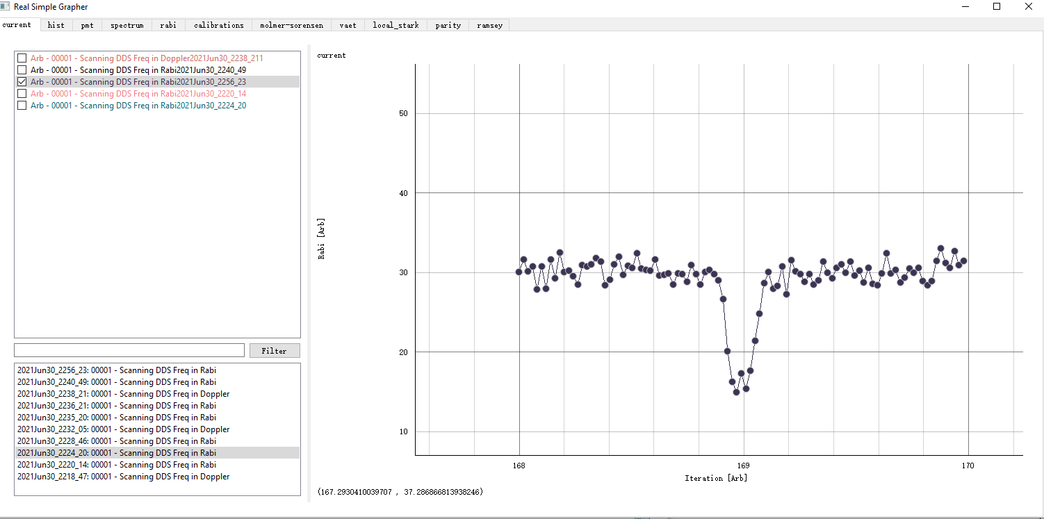
Many of the time we just need a linegraph with an x and y axis. The x axis is the independent variable we are scanning, and the y axis is the data representing some features of this point. In this case, we usually need to pre-process the data in a scanning point into a single value integer. For example, we can just do an average (e.g. compute probability of a bright state), or we can calculate some correlation (e.g. parity between two ions). We will send a list of two points of [scannvalue, result] to the datavault of a dataset, and then the grapher can display the data, just as an example showed below.

Histogram

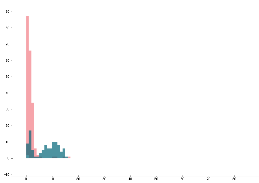
Another type of data is the histogram. A single average we talked above can be deceiving. For example, if we are using the PMT to detect the state of the ions, how do we know that after averaging, a value that is half of the bright state count is refer to 1: 50% of the bright state rather than 2: the ions are always in bright states and it is just the detection light becomes dimmer? As a result, we need to look at the distribution in the form of the histogram. In situation 1 we will see two Posson distributions, one around the bright state count and the other around the dark state count, as shown by the two green distributions in the graph below. Whereas in situation 2 we will just see 1 Posson distribution around the 50% bright state counts. As a result, if we want to display histogram, we usually will fix the experiment at a single parameter. We will then send a (a list of) data point to the datavault and the datavault will keep updating it(them) on the histogram.

Images

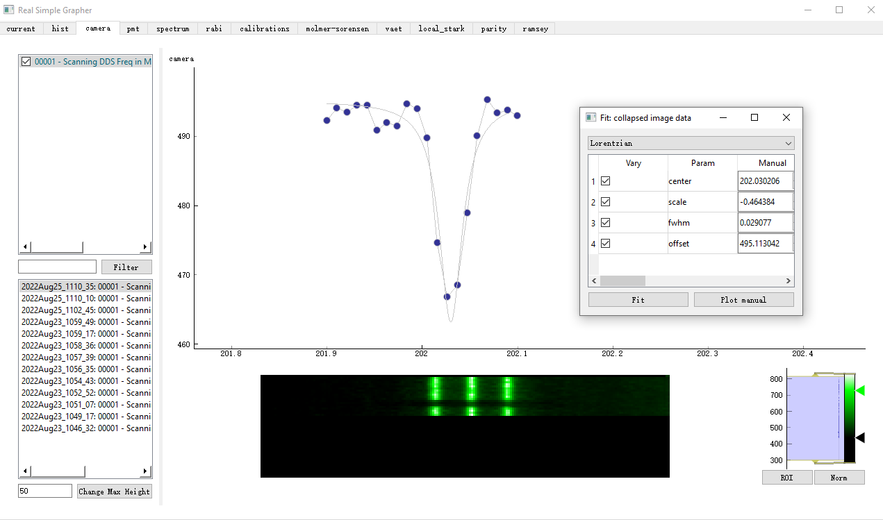
When we have camera in the experiment, we can use the camera data to detect a chain of ions' states. We also want this to be displayed in real time. So we display a two-dim pixel image for our purposes. We have an image of WxM, for W is the length of the image and M is the number of the points we scan. For every scanning point, we do an average of N images into one image and take another average over the vertical axis so that we end up with a Wx1 array. We then send this Wx1 array to the datavault and the grapher will update a row of Wx1 array for every point we scan, thus generating a WxM image that shows the ions' state change over our scanning process. You can see that there is a dip in the middle where 0/3 of the ions are bright, where it corresponds with the linegraph in the top part of the graph when we hit the transition freq during the scanning.

Data Pipeline

In the play ground page we talk about a simple data pipeline with PMT of a toy experiment. In the how to run an experiment we talk about the structures of an experiment execution, and you might remember we implement the data pipeline in the run functions in the middle layer classes (e.g scan_1D_camera). The graph below shows an illustration of what we know so far.

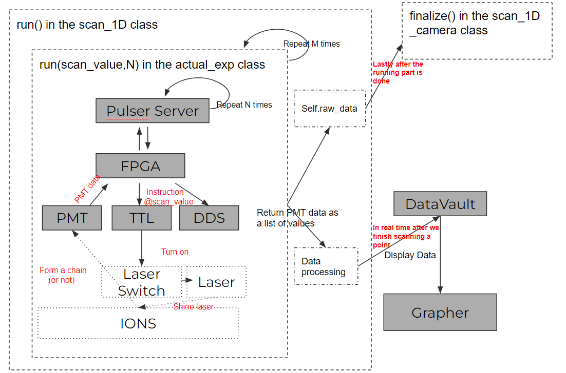
So continue from the background, now we will talk more in details of how we complicated the data pipelines and what we needed to do in order to build new data pipelines. For example, the data process functions in the run function in the scan_1D class can be further implemented. With the PMT data, it is just simply taking an average of N points and send [scannvalue, result] to the datavault. With a camera data, we have to do more averaging and send a Wx1 array to the datavault. With different data types, we also have to call(or imeplement) different functions of the datavault so that the datavault know how to handle them. Note that now we are only using dataset class (there are two fields though, one for array and another for linegraph and different functions update different fields of a dataset) rather than image class. It seems that dataset class is okay for the size of the data we are handling now, image class are needed if we need somehow send raw data to the datavault as the hdf5 format can compress huge data better.

There might be new data type and new ways of display needed, and then one should need to update rsg (probably open up a new section-page like histrogram, camera...) and also implement the functions above to build the new channel for the data pipeline.

Another big part of the data pipeline is the pre-calculation process (especially for awg). This is usually done in the initialize/run functions in the real experiment class. Feedback controls (not in circuit) can be implemented to close the loop by updating the parameter vault in the run/finalize functions in the real experiment class to close the loop. For in circuit feedback control one should implement the HVI functions of the keysight AWG to push the logic in the initialize/run functions in the real experiment class so that the TTL triggers in an experiment can call different logic of the AWG during a single-shot.