Labrad Playground

Although having learnt about the sever/client structure, you might still be confused how labrad is used in reality. In this page, we talk about how you combine with different servers/clients to do simple tasks and get familiar with the system. Usually to run any job, we need a server to provide services and a client to display/save/request tasks. This makes a simplest three layers structure that occurs in Labrad. The fig below illustrates a rough idea how different server/client makes the three layers of labrad where you use your pc to control different instruments.

Start with Datavault and Real Simple grapher.

Although you can start the labrad even without any servers, you still need to run some basic servers and clients to get it do something. We always start with some simple data storing and display features first (basically manually record data from an imaginary experiment and get the "fake" data display and saved).

Fig above shows the structures and the servers/clients used when we want to do the task described above. Note that when dealing with actual tasks servers/clients are more in a structure like graph here instead of the graph above(as it is too general). In order to do that, we need to start real simple grapher(RSG) and datavault and create a new dataset. We can then add data to datavault and also select the data in RSG. All these operations can be found in the datavault and RSG wiki respectively. You can also try to fit the data using RSG. The fig below shows the a Gaussian fitting of some "fake" data we added into the datavault(on a linux PC so UI might look a bit different).

Add a Pulser into the system: A toy experiment

With a pulser added into the system, things become more interesting and more like an experiment. For simplicity, we first talk about how to run the servers with only a pulser server with PMT connected, the datavault server, and the grapher client. The graph below shows a detailed version of the pipelines between the servers/clients when running this setup.

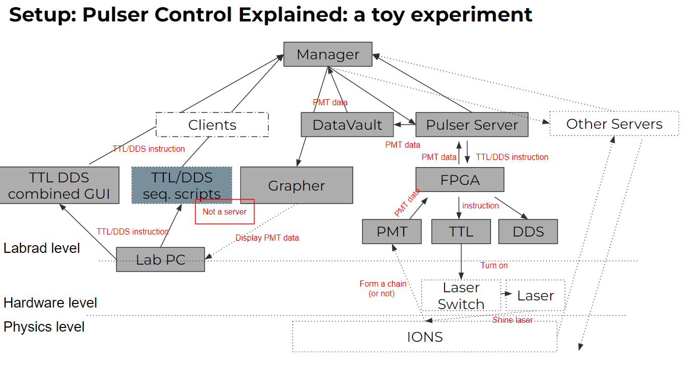
Note that there are two ways to control the pulser. One way is to use the TTL/DDS GUI, which is a client program combined the TTL GUI_and DDS GUI. In this GUI program, you can control the state of the TTL and DDS channels, and their current states (if set by the script codes or other users) will also be reflected in real time. This is a simple way to debug, test the experiment and to do simple TTL/DDS tasks such as loading the ions (by opening the ablation TTL), raise/lower trap voltages etc. But note that using the client GUI you can only change the state of the channels, you cannot generate pulses. The other way, which is using script codes, enables you to control both the states of the channels and generate pulses that are vital to our experiments. For the script details, check out the pulser page. 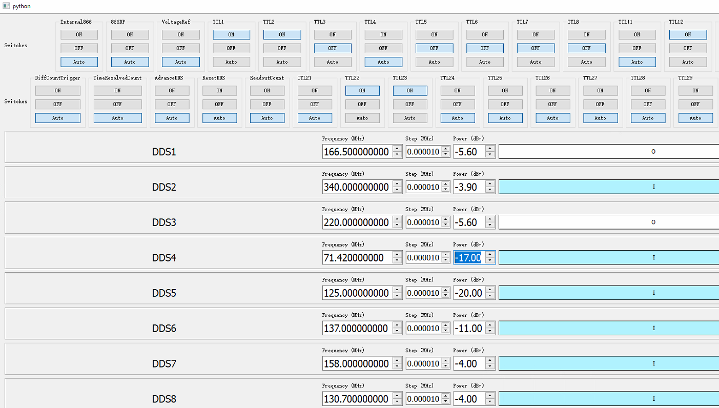A combined GUI for TTL states(open/off/automatic control) & DDS states(on/off/amp/freq/phase)

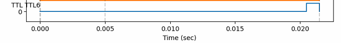
A TTL pulse example in an experiment

A PMT GUI example (we do not use the GUI in this pipeline though), the number in the middle is the photons collected

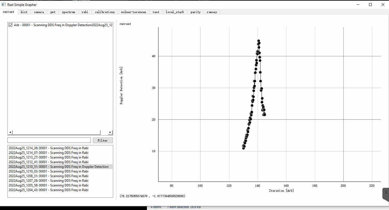An example of RSG displaying real data collected by PMT

Once you give commands to the pulser server, it controls an Opalkelly FPGA and it talks to the TTL and DDS channels that connects to the hardware instruments for the experiment such as switches, AOMs triggers ports for AWGs, or motors, and a photomultiplier tube detector (PMTs). These instrument either detect the ions(PMT), or controls the ions(the rest examples above). For an example experiment, one might use the switch to turn on the laser cooling laser, and then use PMT to detect if the ions are in the trap or not. The PMT will collect the data, then send it to the datavault server, and then the datavault will notify the grapher so that the grapher can display the data. It completes our first data pipeline of a simple toy experiment, while real world experiments with more complicated data pipelines will be introduced in the following sections.