Make Z calibration - UU-cellbiology/DoM_Utrecht GitHub Wiki

This page contains step-by-step description of Z axis (astigmatism)^{(check it first)} PSF calibration. Usually, this procedure is iterative, meaning you'll probably need to try it a couple of times, before getting optimal results (especially on the very first try).

Before running this wizard, as an input, you'll need to prepare a Z-stack of point spread function (PSF). For this purpose, usually you need a sample with some sub-diffraction objects (Tetraspeck beads, quantum dots, etc). The calibration will be more reliable if these beads are located on the same coverslip as the imaged sample. In principle, a Z-stack of a single bright bead can be used, but it is better to use averaged image of the PSF. For that, we wrote short Extracting 3D PSF instructions.

Ideally, this Z-stack will be cropped in all dimensions so that there is a single PSF located at its center:

Once you have this data, open it in ImageJ/FIJI and go to

Analyse -> DoM vX.X.X -> Z axis (astigmatism) -> Make-Z-calibration

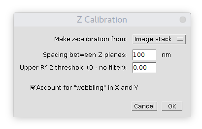
The following dialog should be displayed:

To create a calibration, the plugin needs to detect and fit an image of PSF at each slice on Z-stack. In case there is more than one detection per slice, the plugin first will perform "tracks" linking. Then it will use only the longest track detections (spanning most of the slices) as a calibration input.

So the first parameter "Make z-calibration from" defines if the calibration will be made directly from the Z-stack (Image stack) by detecting/fitting spots. In this case, after clicking "OK" button, the plugin will prompt a Detect Molecules dialog. The detections will be automatically linked to a track using a displacement value of 4 pixels.

Sometimes it is more convenient to perform detection in advance and try different detection/linking parameters. For this case, one can choose "Particle Table" value, the plugin will load detections/fittings directly from the current Results table. This method allows tweaking Link Particles to Tracks parameters manually. Again, only the data from the longest track in the Results table will be used.

The second parameter "Spacing between Z planes" is, well, the distance between z planes of the calibration data, i.e. Z-step of the stage during beads acquisition.

The third parameter "Upper R^2 threshold" allows filtering poorly fitted spots based on the "goodness of fit" criteria.

The last parameter "Account for "wobbling" in X and Y" allows to compensate for the change of lateral (XY) coordinates along Z axis (we recommend to use it).

After clicking "OK" button, in case of "Image stack" option, a detection dialog should appear. If you use "Particle table", the plugin will proceed straight to the fitting.

This dialog performs Z calibration fitting. Upon the start, the following window is displayed:

The left top plot displays the width and the height of the PSF at each slice (Z position). The bottom left plot shows the subtracted values. This is the data that will be fitted and the fit will be later used to calculate z-coordinate.

Two plots on the right side depict changes in X and Y coordinates along the z-axis and will be used for "XY wobbling" correction. These values will be always fit with the polynomial of 4th degree and it cannot be changed.

The parameters on the top of the dialog specify the fitting range and the position of zero Z. The data from the left bottom plot will be fitted with a polynomial function y=P(x) with a degree, specified by the parameter on the top right corner of the dialog (1, 2 or 3).

In spite of the appearance of the bottom left plot, the fitting treats PSF's (width-height) as a polynomial x coordinate and Z position as a y coordinate. Later, at the Calculate Z values stage, the plugin will put the value of an individual spot (width-height) into the fitted polynomial and get its Z position.

Therefore it is a good idea to limit the fitting range to the monotonous part of the function displayed at the left bottom and exclude (usually) dim and unreliable spots at its sides. The Z zero position is usually chosen at a point where the absolute value of PSF's (width-height) is minimal (it is automatically estimated by the plugin in the initial stage).

To find the fit, you need to press "Perform Fit" button and the fitted plots should be displayed together with a standard deviation (well, actually RMS) of difference between the data and the fit.

In case the fit does not look good, one can adjust Z range and zero parameters and press the "Perform Fit" button again.

If you are satisfied with the fit, press "Store calibration", it will be saved to the ImageJ registry and will become the current active calibration. So whenever you need to calculate Z values, the plugin will not ask you for the calibration, it will just use the one that is currently stored (and it can be only one that is stored). If you restart ImageJ/FIJI (as well as the computer), this calibration will still be there.

Again, you can save and load calibration as a text file for reference and future use.