Selecting Optimal Filters with ERPLAB Toolbox - ucdavis/erplab GitHub Wiki
Using an appropriate filter can dramatically increase your effect sizes and your statistical power. However, an inappropriate filter can dramatically distort your ERP waveforms, leading to bogus effects and completely false conclusions. The optimal filter settings will depend on the nature of your research participants, the kinds of experiments you run, the quality of your recording setup, and the specific amplitude or latency scores that you will be analyzing. How can you determine the optimal filter settings for your data?
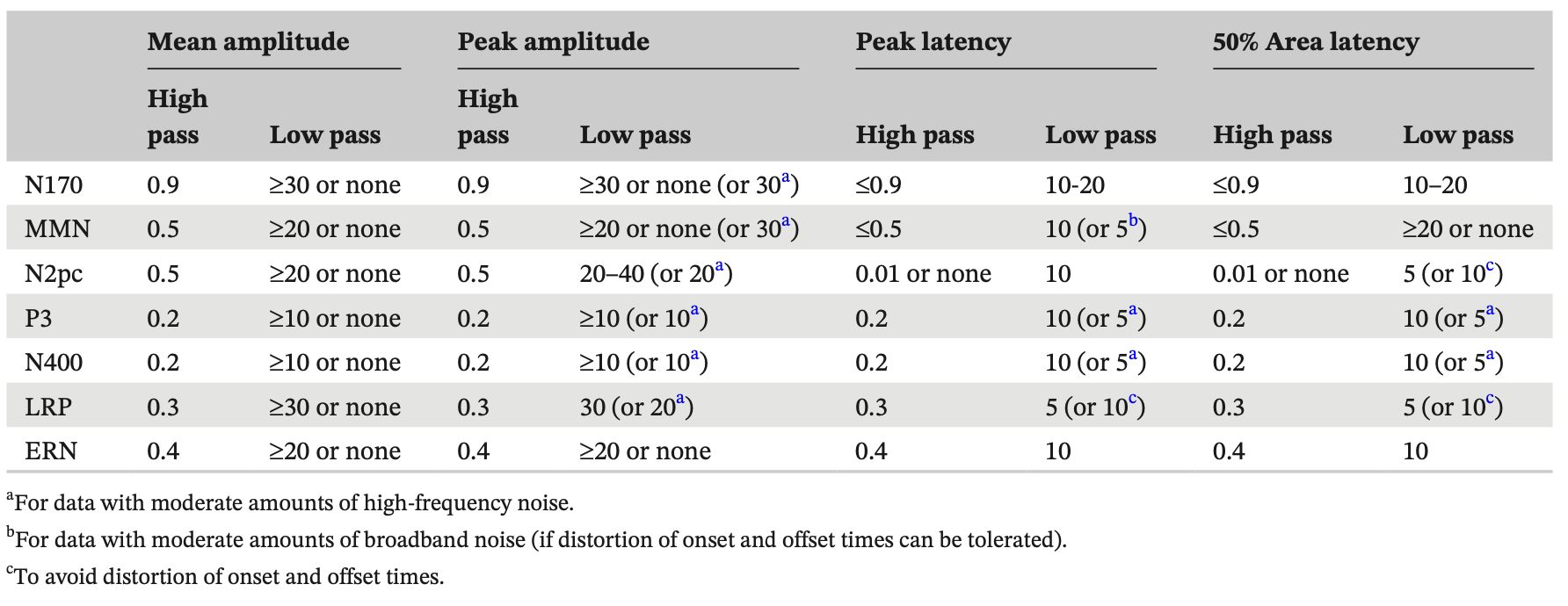
We have developed an approach for selecting optimal filter settings, along with ERPLAB tools that make it relatively simple for you to apply this approach to your own data (Zhang et al., 2024a). We have also applied this approach to the ERP CORE, which includes data from 40 healthy young adults who performed six standardized paradigms that yielded seven commonly-studied ERP components. If you are analyzing reasonably similar data, you can simply use the settings we developed using the ERP CORE data (Zhang et al., 2024b), as shown in the table below.
If your study is a bit different from the ERP CORE, these settings should still be reasonably close to optimal for your data. However, if you are using a very different participant population (e.g., young infants), a very different recording setup (e.g., dry electrodes), or very different ERP components (e.g., auditory brainstem responses), you may need very different settings. The purpose of this document is to explain exactly how to use ERPLAB to determine the optimal settings for your data. This will take a fair amount of time, but once you have done it, you can use the same filter settings for any reasonably similar dataset.
As described in Zhang et al. (2024a), we define the optimal filter as the one that maximizes data quality while minimizing waveform distortions. Our approach begins by applying a large number of filters with different low-pass and high-pass cutoff frequencies to a given dataset to quantify the data quality yielded by each filter. We then assess the amount of waveform distortion produced by each filter. We then select the filter that produces the best data quality without exceeding a threshold for waveform distortion.
Our approach to quantifying data quality uses the standardized measurement error (SME), which assesses the noise level of a given participant’s data with respect to a specific amplitude or latency score. A smaller SME means lower noise, and filters generally decrease the SME. You can read more about the SME at:
- Blog post: A New Metric for Quantifying ERP Data Quality
- Published papers:
For latency scores (e.g., peak latency, 50% area latency), we simply use the SME to quantify the data quality resulting from a given filter. For amplitude scores (e.g., peak amplitude, mean amplitude, area amplitude), a filter may reduce the score (the signal) in addition to reducing the noise, and it is important to assess the reduction in noise relative to the reduction in signal. Thus, our approach uses the signal-to-noise ratio (SNR) to evaluate the effects of filters on amplitude scores. The signal is defined as the score itself, and the noise is defined as the SME for that score. When the SNR is quantified in this manner, we refer to it as the SNRSME.
Whenever possible, we recommend using difference waveforms (e.g., rare-minus-frequent for the P3 wave, faces-minus-cars for the N170, contralateral-minus-ipsilateral for N2pc and LRP) to assess waveform distortion and quantify the signal and the noise. This will allow you to assess how the filter impacts your experimental effect and decide on a single filter for all experimental conditions. If you are studying multiple groups, you should collapse across groups as well so that you can decide on a single filter for all groups.
Filters inevitably distort ERP waveforms, and our approach involves quantifying the amount of waveform distortion. We do this by creating a simulated waveform that resembles the effect of interest and examining the distortion produced when this waveform is filtered. It is necessary to use simulated waveforms rather than real data to assess waveform distortion because the true waveform is not known for real data. The most problematic type of waveform distortion produced by typical ERP filters is the introduction of artifactual peaks before or after the true peaks. We quantify this by computing the artifactual peak percentage, which is the amplitude of the artifactual peak as a percentage of the amplitude of the true peak (after filtering).
We recommend quantifying waveform distortion first. This step is relatively simple and fast, and it will allow you to focus the more time-consuming steps on filters that create acceptable levels of distortion. To assess waveform distortion, you must create an artificial ERP waveform that approximates the true waveform. Of course, you don’t know the true waveform, but the simulated waveform does not need to be an exact match.
You can create a simulated waveform in ERPLAB Studio (using the Create Artificial ERP Waveform panel in the ERP tab), in ERPLAB Classic (using ERPLAB > Create Artificial ERP Waveform), or using a Matlab script (see example at: https://osf.io/98kqp/). These tools allow you to create a Gaussian waveform (which is good for most perception- related components) or an ex-Gaussian waveform (a skewed version of a Gaussian, which is good for most cognitive components). The function allows you to overlay the artificial data with a real ERPset (usually a grand average difference wave) so that you can visually adjust the parameters of the simulated waveform until it matches the real data. If the real waveform is complex (e.g., a negative-going ERN followed by a positive-going Pe), you can either try to simulate one portion of if (e.g., just the ERN), or you can simulate multiple components individually and then sum them together (by saving each waveform in a separate file, appending them together, and then summing them using Bin Operations).
The next step is to apply each filter you would like to test to the simulated waveform. You can apply a given combination of low-pass and high-pass filters simultaneously. Ordinarily, it’s not a good idea to apply high-pass filters to averaged ERP waveforms because of the potential for edge artifacts. However, this will not be a problem with artificial data as long as you simulate a sufficiently long epoch (e.g., -2000 to +2000 ms) and make sure that the simulated component reaches zero well before the beginning and end of the epoch.
If you plot the filtered waveforms, you should be able to see the distortion produced by the filter (hint: if you want to overlay the filtered and unfiltered waveforms, you must first append them into the same ERPset). You can then quantify the amplitude distortion using the Measurement Tool. You will want to find the positive peak amplitude over the entire epoch and find the negative peak amplitude over the entire epoch (for the filtered waveform). These numbers can then be converted into the artificial peak percentage, which is 100 times the absolute value of the peak voltage of the artifactual peak divided by the absolute value of the peak voltage of the true peak. For datasets recorded from highly cooperative subjects (e.g., college students) using a high-quality recording system in most standard paradigms, we recommend using filters that produce less than 5% distortion. For much noisier datasets, a higher threshold would be reasonable.
The next step is to quantify the noise using the SME for each filter you wish to consider. You will obtain an SME value from each individual participant, and then you will aggregate across individuals using the root mean square (RMS) of the single-participant values. See the Manual Page on Data Quality Metrics for detailed information about how to compute the SME in ERPLAB. You should apply all of your usual preprocessing steps (e.g., re-referencing, filtering, artifact correction/rejection) prior to computing the SME. You will therefore need to preprocess your data separately for each filter you wish to test. If you are using ICA-based artifact correction, we recommend computing the ICA coefficients once and then transferring them to each filtered dataset before removing the artifactual components (see Chapter 9 in Luck, 2022).
SME for mean amplitude scores ERPLAB makes it easy to compute the SME values for mean amplitude scores. When you average the data using ERPLAB > Compute averaged ERPs, you simply select “On – custom parameters” in the Data Quality Quantification section of the averaging GUI, and customize the aSME data quality measures to include the time window that you are using to compute your mean amplitude scores (e.g., 300-600 ms for the P3 wave). The ERPset created by averaging will then contain the SME values for this time window. To get the SME value for a difference between two conditions, you can use this equation: SMEA-B = sqrt(SMEA2 + SMEB2). SMEA-B is the SME of the difference between conditions A and B, and SMEA and SMEB are the SME values from the two individual conditions. Note that this equation applies only when the score is the mean voltage across a time window and when the difference wave is between waveforms from separate trials (e.g., rare minus frequent for P3, unrelated minus related for N400). You must instead use bootstrapping if you are scoring a difference between two electrode sites (e.g., contralateral minus ipsilateral for N2pc) or looking at some other score (e.g., peak amplitude, 50% area latency).
Bootstrapped SME values If you are unable to use the simple approach described in the previous paragraph, you can instead using bootstrapping to obtain the single-participant SME values. At present, this requires scripting. You can find an overview of how to compute bootstrapped SME values in Luck et al. (2021), and you can see example scripts at https://osf.io/a4huc/. You can learn how to write EEGLAB/ERPLAB scripts by reading Chapter 11 of Luck (2022).
Choosing electrode sites You will get separate SME scores for different electrode sites. In terms of selecting an optimal filter, the exact electrode site shouldn’t matter much, and the simplest thing to do is to use the channel in which the effect is largest. You could also collapse across a set of channels prior to averaging (using Channel Operations) to create a clustered channel, and then you could obtain the SME value from this clustered channel.
Aggregating across participants Once you have the single-participant SME scores, you can combine them into a single RMS(SME) value by squaring the SME values, summing the squared values together, and then taking the square root of this sum.
For amplitude scores, you will need to take the RMS(SME) value from the previous step and use it to compute the SNRSME. This is quite simple. Using ERPLAB’s Measurement Tool, you simply measure the score of interest from the grand average waveform (preferably a difference waveform). This is done separately for each filter you are evaluating. The SNRSME for a given filter is then computed by dividing this score by the RMS(SME) value for that filter. You do not need the SNRSME value when dealing with latency scores. You will simply use the RMS(SME) value.
For amplitude scores, you will select whatever filter produced the largest SNRSME value while not exceeding the maximal acceptable artificial peak percentage (e.g., 5%). For latency scores, you will select whatever filter produced the smallest RMS(SME) value while not exceeding the maximal acceptable artificial peak percentage (e.g., 5%).