Step 5: Count Mapped Reads - srkoppolu/SK_RNA-Seq GitHub Wiki
After aligning the sequence reads to the reference genome/transcriptome and ensuring the quality of the aligned reads, the next step is to count how many reads have mapped to each gene/transcript. There are numerous tools that perform this task of counting the number of reads (counts) associated with each feature of interest (genes / exons / transcripts / ...). Two of such most commonly used counting tools are: featureCounts and htseq-counts.
These tools work best in counting at the gene level as they report only the "raw" counts that map to a single location (unique mapping). Total read counts to a gene is equal to the sum of the read counts to each of the exons belonging to that gene. In this case, the counts would always be whole numbers. There are also other tools that can account for multiple transcripts for a given gene, in which case the counts can be fractions and not necessarily whole numbers. Although some tools have the ability to do multimapping reads, they are to be cautiously as there is the possibility of overaccounting the total number of reads which can cause issues with normalization and skew the DGE results.
Generally, for counting the mapped reads, the input and output are as follows:
- Input: multiple BAM files (genomic coordinates of where the reads are mapped) + 1 GTF file (genomic coordinates of the interested feature (exons / transcripts / genes).
- Output: A count matrix (of "raw" counts) with genes across rows and samples across columns.
featureCounts
featureCounts is a highly efficient read summarization tool that counts mapped reads for genomic features (genes, exons, promoter, gene bodies, genomic bins and chromosomal locations). This tool works well for both RNA-Seq counts as well as DNA-Seq counts. It is available as part of the Rsubread package.
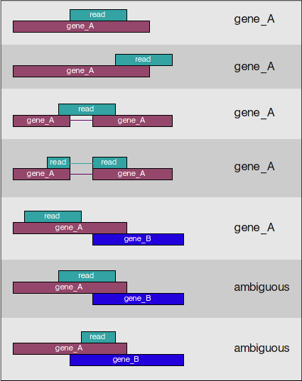
It counts reads that map to a single location (uniquely mapping) and follows the scheme in the figure below for assigning reads to a gene/exon [source].
Note: For featureCounts, specifying the strandedness is very important. When specified, it takes into account the strand in addition to the genomic coordinates.
To run featureCounts using HPC,
first start an interactive session with appropriate number of cores:
# In the srun examples below, through "--pty /bin/bash" we request to start bash command shell session in pseudo terminal
#
# by default the resource allocated is single CPU core and 2GB memory for 1 hour
$ srun --pty /bin/bash

# To request 4 CPU cores, 4 GB memory, and 2 hour running duration
$ srun -c4 -t2:00:00 --mem=4000 --pty /bin/bash

# To request one GPU card, 3 GB memory, and 1.5 hour running duration
$ srun -t1:30:00 --mem=3000 --gres=gpu:1 --pty /bin/bash
Note: Make sure the path for featureCounts is added to the $PATH variable. If it is not already added, add the following export command to the ~/.bashrc file using vim: export PATH=$HOME/bcbio/tools/bin/:$PATH.
Next, run the featureCounts tool...
$ featureCounts -T 4 -s 2 \
  -a /HOME/reference/Homo_sapiens.GRCh38.92.gtf \
  -o ~/rnaseq/results/counts/Sample_1_featurecounts.txt \
  ~/rnaseq/results/STAR/bams/*.out.bam
The general usage for featureCounts is featureCounts [options] -a <annotation_file> -o <output_file> input_file1 [input_file2] .... For the options:
-T 4specifies the usage of 4 cores-s 2specifies that the data are 'reverse'ly stranded
Note: If logging is needed as well, then add the following command after the input_files:
2> /rnaseq/results/counts/Sample_1_featurecounts.screen-output.log
The output of featureCounts produces two files, one for the count matrix and the other for the summary filewhich tabulats how many reads were "assigned" or counted and the reason they remained "unassigned".