Fluid_State_Error - nasa/gunns GitHub Wiki
{{>toc}}
Because of an assumption in the GUNNS fluid aspect design, fluid capacitive nodes typically carry a small discrepancy between the fluid mass in the node (the node’s mContent.mMass) and the value given by the product of the node’s volume and fluid density. We call this error the “State”, “Pressure”, or “Mass” error depending on where you look.
We will explain where this error comes from, the issues it leads to, and how GUNNS corrects it.
When GUNNS propagates a fluid network, node mass and pressure are propagated separately and not forced to agree by the fluid’s equation of state. Mass is not1 re-calculated from pressure and vice-versa. Instead, mass is incremented from its previous value by the mass flow rates coming into or leaving the node, and a new pressure comes from the solution to the network’s system of equations. These two propagations generally agree but the assumption below can cause a discrepancy between them to grow.
When GUNNS solves for the new pressure in a capacitive node, it assumes that the fluid compressibility is constant over the time step — that is, the fluid compressibility at the end of the step will be the same as the value used in the solution. However, fluid compressibility isn’t really constant, because fluid density is typically a function of both pressure and temperature. Mass flows into the node resulting from the new network solution can cause the node’s compressibility to change. If the incoming flow has different properties, particularly temperature or mixture, then when it mixes with the fluid already in the node, the resulting mixed node content has a different temperature or mixture, and thus compressibility, than what the new pressure was solved for. The solver can’t know what this new compressibility will be ahead of time, so it can only assume that it will remain the same.
The new node content fluid density is computed to satisfy the fluid’s equation of state at the new pressure, temperature & mixture. However the new mass divided by the node volume doesn’t result in the exact same density value. The node computes this discrepancy and stores it in its mMassError term:
////////////////////////////////////////////////////////////////////////////////////////////////////
/// @details  This method calculates the discrepancy between the theoretical node mass represented
///           by the fluid properties (density) and the actual mass.  This discrepancy arises from
///           the linearizations of pressure and temperature in the network solution, and it is
///           corrected for later so that mass is conserved.
////////////////////////////////////////////////////////////////////////////////////////////////////
inline void GunnsFluidNode::computeMassError()
{
    mMassError = mContent.getMass() - mContent.getDensity() * mVolume;
}
Do not be confused by the mMassError terminology. This is not the error in our actual mass. Rather, this is the amount of mass represented by the error in the fluid pressure and density properties.
Let’s look more closely at an example case that demonstrates this error. We have a very simple network containing two tanks, tank1 and tank2. They both contain 100% pure N2 gas, but at different pressures and temperatures. tank2 has a higher pressure and temperature, and will flow into tank1. tank1 will experience a state error because the incoming flow from tank2 has a different temperature than its original contents. Both tanks have a volume of 1.0 m 3.
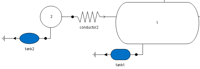
These are values recorded before and after a step from an actual sim with this case set up in a network:
Starting Conditions (t = 0.0):
| term | tank2 | tank1 |
|---|---|---|
| Capacitance (kg*mol/kPa) | 3.436349123723821E-4 | 4.147317907942592E-4 |
| Pressure (kPa) | 200.0 | 101.325 |
| Temperature (K) | 350.0 | 290.0 |
| Density (kg/m3) | 1.925276450850655 | 1.177198667825085 |
| Actual Mass (kg) | 1.925276450850655 | 1.177198667825085 |
| Mass Error (kg) | 0.0 | 0.0 |
After 1 Step (t = 0.1):
| term | tank2 | tank1 |
|---|---|---|
| Capacitance (kg*mol/kPa) | 3.436349123724021E-4 | 4.147314652838589E-4 |
| Pressure (kPa) | 199.9995935788039 | 101.3253367489907 |
| Temperature (K) | 350.0 | 290.0002276123981 |
| Density (kg/m3) | 1.925272538484868 | 1.177201656240208 |
| Actual Mass (kg) | 1.925272538484868 | 1.177202580190871 |
| Mass Error (kg) | 0.0 | 9.23950663089812E-7 |
The flow rate through conductor2 at t = 0.1 is 3.91236578695466E-5 kg/s. Its conductance is 1.0E-7 m 2 and its admittance was 1.415369281617471E-8 kg*mol/kPa/s.
An algebraic solution for this case is given here. It gives the same answer for the node pressures after the step as recorded above. The flow rate through conductor2 should come from the generic GUNNS conductance equation:
w = A*dP
Where A is admittance and dP is the delta-potential (pressure). This equation gives the same flow rate as recorded above (make sure to convert molar flow to mass flow by the fluid’s molecular weight, which is 28.0153 1/mol for N2). The tank masses should have changed by this flow rate multiplied by the time step (0.1 second) — this is the Backwards-Euler (rectangular) integration we do for integrating mass flow. The recorded masses after the step match this amount. The new tank1 density recorded above comes from the N2 fluid properties as a function of the new pressure and temperature, NOT from the new mass divided by the volume. Notice how the density and mass match after the step for tank2 but not tank1. This is because the temperature changed in tank1 but not tank2, and it is the temperature change that causes the discrepancy between the mass and density because, as stated above, the pressure solution for the tanks assumes a compressibility (embedded in the capacitance) that is constant with temperature.
As you can see, the magnitude of the mass error after one step was on the order of 10 7 times smaller than the actual mass, so this is a pretty insignificant error. However this error will compound to significant levels over time as the flow continues in a consistent direction, so it is important to actively correct the error.
Note that the total actual mass at both times is exactly the same, because actual mass is conserved. There are cases where mass isn’t conserved, discussed here: Errors_in_Fluid_Conservation.
A common cause of very large mass errors in a node is a link that fails to transport fluid mass flow corresponding to the link’s effect on the system of equations. If conductor2 in the above example failed to transport the mass, then the node pressures approach each other, acting like mass is being transported between then, but the actual node masses would remain constant — this would create a very rapid rise in the mass error, much larger than the temperature or mixing causes described above.
Usually when you see very large and rapidly increasing mass errors, it points to such a mistake in the link design or code.
- Excessive state error can lead to oscillation & instability in the network as the nodes try to correct it.
- This discourages us from mixing non-ideal gas fluid types. The compressibility of different ideal gases changes at exactly the same rate, so when we change ideal gas mixtures, no error results. Other fluid types don’t behave this way. This is the reason we discourage mixing multiple liquid types in the same node; large state errors result. Similar errors occur when mixing a non-ideal gas, such as GUNNS_O2_REAL_GAS, with ideal gasses.
- If not corrected, the error can grow until it becomes obvious to the user. Mass flows are a function of pressure, not mass itself. Continuously growing error can result in negative mass in a node even though the pressure appears perfectly normal, and flow continues! A user inspecting the node will see negative mass which is an obvious sign that the model isn’t working.
Another way of looking at the state error is as an error in pressure. The actual pressure from the network solution will disagree with the PVT state equation pressure (as a function of density, temperature, and mixture) for the resulting node fluid contents, after the incoming fluid flows have been mixed. The node finds this error in pressure in order to correct the error (described in more detail below) as:
double GunnsFluidNode::computePressureCorrection()
{
    .
    .
    .

        /// - The node density and pressure will disagree with the mass.  Calculate the ideal
        ///   (correct) density and pressure from mass, volume, and temperature.  The pressure error
        ///   is the difference between this pressure and the current node pressure.
        const double idealDensity  = mContent.getMass() / mVolume;
        const double idealPressure = mContent.computePressure(mContent.getTemperature(),
                                                              idealDensity);
        const double pressureError = idealPressure - mContent.getPressure();
In the above code, mContent.getPressure() is the network’s pressure solution. Note that “ideal” in the above variable names does not imply Ideal Gas Law, but rather what the correct values should be. This stuff is agnostic to the fluid state equation. The idealPressure term is what the pressure ought to be based on the actual mass in the node. Since we go to great pains to conserve mass as we transport it around a network, we consider the actual mass in the node to be correct, and the mass given by fluid density * volume to be incorrect. Likewise, we consider idealPressure to be the correct value, and the network’s pressure solution as incorrect. In other words, when the node’s mContent.mPressure disagrees with mContent.mMass, we consider the mass to be correct and the pressure in error.
The GunnsFluidCapacitor link, in its step method, calls the node’s computePressureCorrection() to get the value of the pressure correction to use to correct the state error. The correction value is added to the last-pass pressure of the node in the link’s source vector term. Whereas the capacitor’s contribution to the system of equations for the capacitive node is normally:
[A]·{p} = {w}
[C/dt]·{p t~} = {(p ~t-1)·C/dt},
the pressure correction p c is included as:
[C/dt]·{p t~} = {(p ~t-1 + p c)·C/dt}.
The sum of (p t-1 + p c) is the corrected node pressure — it approaches what the actual pressure ought to be based on the current mass, temperature & mixture in the node. This causes the subsequent network solution to propagate from the corrected pressure instead of the previous erred pressure solution. Repeating this process every pass causes the state error to wash out over time.
The pressure correction applied by the capacitor is not exactly equal to the node’s pressure error at any instant in time. Instead, the correction is a low-pass filter of the error. The filter gain cuts out rapidly when the node pressure oscillates, and rises slowly to its full value when there is no oscillation. This prevents instability in the network when multiple nodes are correcting their errors at the same time.
The resulting behavior of the state error is a sudden growth when an un-mixed (different temperatures/mixtures) flow starts, followed by a damping and slow wash-out of the error when the system reaches steady-state or comes to rest. The following chart shows the Node 1 mass error and pressure correction over time from the above example:

The magnitude of pressure correction you’ll typically see depends on many factors and what kind of fluid system you are modelling, but it’s typically damped to less than 1 kPa unless you have a very dynamic system. Historically, we tend to ignore corrections < 1 kPa as normal GUNNS behavior, and only worry about possible problems when we see larger corrections.
1 In the normal propagation of a network, most links, including fluid capacitors, do not directly compute mass from pressure & vice-versa. Exceptions are during sim initialization, restarts & some user edits, particularly when changing node volume.