Black line detection with OpenCV - mktk1117/six_wheel_robot GitHub Wiki
In this page, a line detection algorithm is considered.
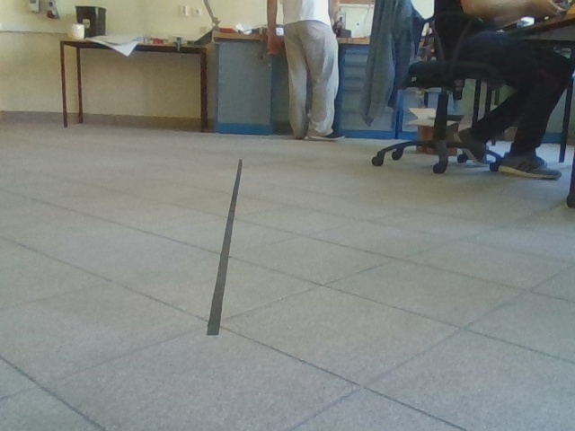
The objective is to recognize where is the black line in the image like this.
First, calculate the distance between RGB because the black color's value of R, B and G seems to be equal. The distance can be calculated by

If this value is small, the pixel is considered to be similar to black. Then, define the black_ratio as below.
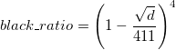
Then, first calculate the grayscale value
grayscale = 0.3R + 0.59G + 0.11B
and, calculate the each pixel value with the equation below
pixel = (255 - grayscale) x black_ratio
void LineDetector::extract_black(Mat* src, Mat* dst, double th_g){
    // loop for each pixel
    // skip some pixels to calculate fast
    for(int y = 0; y < src->rows; y=y+skip_step_){
            for(int x = 0; x < src->cols; x=x+skip_step_){
                    double r = src->data[ y * src->step + x * src->elemSize()];
                    double g = src->data[ y * src->step + x * src->elemSize() + 1];
                    double b = src->data[ y * src->step + x * src->elemSize() + 2];

                    // calculate the distance between R, B and G
                    double distance = sqrt((r - g) * (r - g) + (r - b) * (r - b) + (g - b) * (g - b));

                    // black_ratio = (1 - distance / 411)^4
                    double black_ratio = 1 - (distance / 411);
                    if(black_ratio < 0){
                        black_ratio = 0;
                    }
                    black_ratio = black_ratio * black_ratio;
                    black_ratio = black_ratio * black_ratio;

                    // grayscale
                    int gray = 0.3 * r + 0.59 * g + 0.11 * b;
                    int p = (255 - gray) * black_ratio;

                    // binarize
                    if(p > th_g){
                        dst->data[ y / skip_step_ * dst->step + x / skip_step_ * dst->elemSize()] = 255;
                    }
            }
    }
    return;
}The result of the extracting black part is like below.
Then apply sobel filter to the black image.
Mat black_image = Mat::zeros(Size(org.cols / ld.skip_step_ + 1, org.rows / ld.skip_step_ + 1), CV_8U);
ld.extract_black(&org, &black_image, 130);
Mat filteredx = black_image.clone();
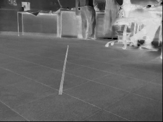
Sobel(black_image, filteredx, CV_8U, 1, 0);The result is like below.

After applying the sobel filter, we want to use Hough transform to detect the line.
But, the problem is there are many lines above the horizon line.
So, before applying the hough transform, detecting the horizon line is needed.
To detect, I calculated the variance along the x axis.
Scan from the bottom, and if the variance is higher than a certain threshold, that position can be detected as the horizon line.
void LineDetector::calc_variance(Mat *src, vector<int> *variance, int th, int direction){
    // direction 0 -> x axis, 1 -> y axis
    if(direction == 0){
        // loop for each pixel
        // skip some pixels to calculate fast
        for(int y = 0; y < src->rows; y=y+skip_step_){
            int mx = 0;
            int mx2 = 0;
            int n = 0;
            // sum for x axis
            for(int x = 0; x < src->cols; x=x+skip_step_){
                double p = src->data[ y * src->step + x * src->elemSize()];
                if(p > th){
                    mx += x;
                    mx2 += x * x;
                }
                n++;
            }
            // calculate variance
            // V = E(X^2) - E(X)^2
            int v = mx2 / n - (mx / n) * (mx / n);
            variance->push_back(v);
        }
    }
    else{
        for(int x = 0; x < src->cols; x=x+skip_step_){
            int my = 0;
            int my2 = 0;
            int n = 0;
            // sum for y axis
            for(int y = 0; y < src->rows; y=y+skip_step_){
                double p = src->data[ y * src->step + x * src->elemSize()];
                if(p > th){
                    my += y;
                    my2 += y * y;
                }
                n++;
            }
            // calculate variance
            // V = E(X^2) - E(X)^2
            int v = my2 / n - (my / n) * (my / n);
            variance->push_back(v);
        }
    }
}
Use this function to detect horizon.
vector<int> variance;
ld.calc_variance(&filteredx, &variance, 100, 0);

int y_border = 0;

for(int i = variance.size(); i > 0; i--){
    cout << variance[i] << endl;
    if(variance[i] > 30){
        y_border = i;
        break;
    }
}
The result is like below.
Then the last step is applying Hough transform to the image below the horizon line. Before applying I binarized the image.
Mat cutted(filteredx, Rect(0, y_border, filteredx.cols, (filteredx.rows - y_border)));
vector<Vec4i> lines;
HoughLinesP(cutted, lines, 1, CV_PI/180, 80, 30, 8 );
The result is like below.

To use the result of line detection, the problem is that the image is captured from the vehicle camera and the position on the image is different from the position in the real world. To solve this problem, transformation from the vehicle viewpoint image to the top view image is used. ###Homography transform
The Homography transformation is a popular geo-referencing technique used worldwide. It is based on quite complex geometric and mathematic concepts, known as "homogeneous coordinates" and "projective planes", the explanation of which is not within the scope of this document.

####Homography matrix The transformation is based on this formulation,
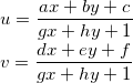
This formulation can be described as below,
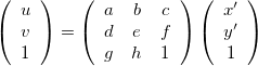
The matrix is called homography matrix.
To calculate the matrix, defining four points is enough
by using getPerspectiveTransform of OpenCV, (Documentation).
In this project, I defined the four point as the figure.

Upper square is cutted image and below square is projected square.
The sample code of calculating using this function is below.
const cv::Point2f src_pt[]={
                cv::Point2f(0, 0),
                cv::Point2f(cutted_org.cols , 0),
                cv::Point2f(cutted_org.cols , cutted_org.rows),
                cv::Point2f(0, cutted_org.rows)};
const cv::Point2f dst_pt[]={
                cv::Point2f(0, org.rows),
                cv::Point2f(0.0, 0.0),
                cv::Point2f(org.cols / 1, 1.5 * org.rows / 5),
                cv::Point2f(org.cols / 1, 3.5 * org.rows / 5 )};

const cv::Mat homography_matrix = cv::getPerspectiveTransform(src_pt,dst_pt)
where, cutted_org is cutted image and org is original image.
![]()
To reduce the computation, this homography transformation is applied only for detected lines. To apply, a function that transform a point can be used.
Vector2d LineDetector::transform_point_homography(Vector2d point){
    Vector3d p(point.x(), point.y(), 1);
    Vector3d t = homography_matrix_ * p;
    Vector2d result(t.x() / t.z(), t.y() / t.z());
    return result;
}
Each detected lines has two points, so use this function and get two transformed points.
   for(unsigned int i = 0; i < lines.size(); i++){
        Vec4i l = lines[i];
        Vector2d p1(l[0] * skip_step_, l[1] * skip_step_);
        Vector2d p2(l[2] * skip_step_, l[3] * skip_step_);
        // transform the point to the floor coordinate
        Vector2d pstart = transform_point_homography(p1);
        Vector2d pend = transform_point_homography(p2);
}![]()
![]()