Section 2 Localization - ika-rwth-aachen/acdc GitHub Wiki

In this workshop, we will perform localization based on GNSS and LiDAR measurements. To achieve a high frequent pose estimate, we will fuse both sources of information.

We will use a recording from a simulation containing LiDAR point clouds, GNSS measurements and a corresponding ground-truth pose. To better understand the context of the vehicle's environment, the recording also contains a stream of camera images.

The learning goals of this workshop are ...

• Set up a localization stack for automated driving in an urban environment using ROS 2
• Utilize and investigate KISS-ICP LiDAR Odometry
• Implement further processing of the lidar odometry output by combining it with low-frequent GNSS measurements
• Apply projections and transformations to the GNSS measurements
• Record a bag file for further investigations of the results in a separate Notebook Exercise

• Combining GNSS and LiDAR-Odometry for frequent pose estimation
• Contents
• Introduction to this workshop
• ROS 2's nav_msgs/msg/Odometry Message
• ROS 2's sensor_msgs/msg/NavSatFix Message
• ROS 2's geometry_msgs/msg/PoseStamped Message
• Investigating KISS-ICP LiDAR Odometry
  • Task 1: Configuration of KISS-ICP
• Processing of GNSS measurements
  • Task 2: Projecting GNSS measurements into the UTM reference frame
  • Task 3: Transforming an UTM point into a local map frame using tf2
  • Task 4: Estimating the vehicle yaw from sequential GNSS measurements
• Combining Odometry and GNSS measurements
  • Task 5: Predicting the current pose using relative odometry measurements
• Result
• Preparation for Notebook Exercise
• Wrap-up

We prepared a rosbag with measurement data captured in simulation for you to use.

Download the file localization.db3 from here (1.2 GB).

Save this file to your local directory ${REPOSITORY}/bag. This directory will be mounted into the docker container to the path /home/rosuser/ws/bag.

After the download, navigate to the local directory ${REPOSITORY}/docker on your host and execute ./ros2_run.sh to start the ACDC docker container.

Inside the container, you can navigate to /home/rosuser/ws/bag and execute ros2 bag info localization.db3 to inspect the rosbag:

Files:             localization.db3
Bag size:          1.2 GiB
Storage id:        sqlite3
Duration:          117.463s
Start:             Sep 26 2023 10:44:22.915 (1695717862.915)
End:               Sep 26 2023 10:46:20.379 (1695717980.379)
Messages:          6051
Topic information: Topic: /camera/image | Type: sensor_msgs/msg/Image | Count: 2375 | Serialization Format: cdr
                   Topic: /gnss/navsatfix | Type: sensor_msgs/msg/NavSatFix | Count: 114 | Serialization Format: cdr
                   Topic: /ground_truth/pose | Type: nav_msgs/msg/Odometry | Count: 2375 | Serialization Format: cdr
                   Topic: /lidar/pointcloud | Type: sensor_msgs/msg/PointCloud2 | Count: 1187 | Serialization Format: cdr

You can see that the rosbag has a duration of 117 seconds and contains 4 different messages:

• A sensor_msgs/msg/Image on topic /camera/image published with a frequency of 20 Hz. The purpose of the image stream is simply to get a better understanding of the environment the vehicle is moving in.
• A sensor_msgs/msg/NavSatFix on topic /gnss/navsatfix published with a frequency of 1 Hz. This topic provides information of the vehicle position in a global reference frame.
• A nav_msgs/msg/Odometry on topic /ground_truth/pose published with a frequency of 20 Hz. This topic is mainly utilized for debugging and evaluation purpose. Keep in mind, that it is really hard to gather ground-truth measurements for pose estimation in real-world. In this case since we captured this bag file using a simulation, we were able to easily derive the actual pose of the vehicle.
• A sensor_msgs/msg/PointCloud2 on topic /lidar/pointcloud published with a frequency of 10 Hz. This topic will be the input for LiDAR-Odometry.

In the context of this course, the nav_msgs/msg/Odometry and the sensor_msgs/msg/NavSatFix will be new to you in particular. In the following, we will briefly discuss these two message types.

The message definition nav_msgs/msg/Odometry is part of ROS 2's standard messages. It is used for indicating an estimate of a robot's (or in our case vehicle's) pose and velocities in 3D space. Within this section, this message type is used for the ground truth pose of the vehicle, and for the output of the LiDAR-Odometry. Please read the documentation about the detailed message format and its content.

The message definition sensor_msgs/msg/NavSatFix is also part of ROS 2's standard messages. It is designed to provide the position derived from any GNSS device. The resulting position is given with respect to the WGS84 system. Feel free to read the documentation about the detailed message format.

The message definition geometry_msgs/msg/PoseStamped is also part of ROS 2's standard messages. It is designed to provide the pose of a robot (or in our case a vehicle) in a cartestian coordinate system. The pose is composed of a geometry_msgs/msg/Point providing the position and a geometry_msgs/msg/Quaternion providing the orientation. For further information on quaternions, please refer to the ROS 2 tutorials.

Now that we've investigated the bag-file, and you gained insights into some of the utilized message definitions, we're ready to build and run some code.

As described above, we will combine GNSS measurements with the output of a LiDAR-Odometry approach to achieve a higher-frequent pose estimate for our vehicle.

Since there are many good implementations publicly available already, the wheel does not always have to be reinvented! In our case, we will use the LiDAR-Odometry pipeline KISS-ICP that is included as submodule (colcon_workspace/section_2/localization/kiss-icp) within our workspace.

We already prepared a launch file to start the lidar odometry within our workspace: colcon_workspace/section_2/localization/localization/launch/odometry.launch.py.

Starting KISS-ICP LiDAR Odometry is as simple as remapping the input topic of the sensor_msgs/msg/PointCloud2 message. To achieve this, adjust the launch-file in line 41.

# START TASK 1 CODE HERE
remappings=[('pointcloud_topic', '/my_pcl_topic')],
parameters=[{
        'publish_alias_tf': False,
        'publish_odom_tf': True,
        'odom_frame': 'odom',
        'child_frame': 'ego_vehicle/lidar',
        'max_range': 100.0,
        'min_range': 5.0,
        'deskew': False,
        'max_points_per_voxel': 20,
        'initial_threshold': 2.0,
        'min_motion_th': 0.01,
    }],
# END TASK 1 CODE HERE

Moreover, you can parameterize the KISS-ICP algorithm with various parameters. Feel free to vary the parameter values later on and observe the influence on the odometry result. For now, you can leave the paremeter values as they are.

When you have successfully edited the launch file and saved your changes, you can navigate to colcon_workspace and build the package with colcon build. Make sure to perform these actions using a terminal window that is attached to your container.

# Run from within the colcon_workspace directory
colcon build --packages-up-to localization --symlink-install

and source the workspace

source install/setup.bash

Now we can launch the LiDAR-Odometry:

ros2 launch localization odometry.launch.py

RViz will open but you won't be able to see anything happen. First, we need to play the bag file. To do so, please attach a new terminal to the docker container with ./ros2_run.sh (if you haven't already).

Again, navigate into the colcon_workspace and source the workspace

source install/setup.bash

Navigate into the bag directory and play the bag-file:

# Run from within the colcon_workspace directory
cd ../bag
ros2 bag play localization.db3 --clock

If everything is configured correctly, the output in the RViz window should look like the following:

The image shows the accumulated pointclouds and the estimated vehicle trajectory (blue line) that is derived via scan-matching through the ICP algorithm.

Investigating the resulting behavior

Inspect the bag file until the end. Maybe you will notice something at the second half of the recording? Can you explain the resulting behavior? Maybe a look at the image stream will help you to explain it!

We'll leave it at that for now since we've successfully launched the KISS-ICP. Feel free to invesitgate the influence of the various parameters on the resulting pose estimate.

In the following tasks, we will combine the output of LiDAR odometry with GNSS measurements to obtain a pose estimate that is as accurate and robust as possible.

The following tasks will all modify the source code of the GNSSLocalizationNode.cpp. First, we will investigate the processing of incoming GNSS measurements. For each incoming GNSS measurement the gnssCallback is called.

Usually, algorithms in an automated driving stack work with cartesian coordinate systems. On the other hand, a GNSS device usually delivers the position estimate with respect to the WGS84 reference system. For this reason, it is necessary to apply a projection from the spherical coordinates to a cartesian coordinate system. In our case, we will use the UTM reference system.

In the respective callback, the incoming message is initially projected to UTM coordinates by the function projectToUTM. We will implement this function in Task 2.

void GNSSLocalizationNode::gnssCallback(sensor_msgs::msg::NavSatFix::UniquePtr msg)
{
  geometry_msgs::msg::PointStamped utm_point;
  // apply projection to get utm position from the received WGS84 position
  if(!projectToUTM(msg->latitude, msg->longitude, utm_point)) return;
  utm_point.header.stamp=msg->header.stamp;
  geometry_msgs::msg::PointStamped map_point;

As already explained in theory, the UTM reference system divides the world into 60 zones. Furthermore, a distinction is made between northern and southern hemisphere. A position within a UTM zone can then be indicated by two values: northing and easting in meters. It is obvious that depending on where we are in the world these values can take large numerical values. For this reason, local coordinate systems are often used, which are defined relative to the UTM zone.

In our case, we're using the carla_map frame which is shifted but not rotated relative to the coordinate system of the UTM zone. This allows us to work with smaller numerical values in the local vehicle environment. In practice, this local coordinate system can be defined, for example, by the segment of the digital map that is used in the vehicle environment.

The transformation from the UTM reference system into the carla-map frame is performed through the function transformPoint. We will implement this function in Task 3.

  // transform the utm-position into the carla_map-frame
  // the corresponding transform from utm to carla_map is provided by the tf_broadcaster_node
  if(!transformPoint(utm_point, map_point, "carla_map")) return;
  // publish the gps point as message
  publisher_gnss_point_->publish(map_point);

Up to this point, we have only considered the position of the vehicle. In addition to the position, the knowledge of the orientation of the vehicle is also required. In this example, we will only consider the 2D pose. Since GNSS does not provide any information about the orientation of the vehicle per se, we will estimate the vehicle orientation from two sequential GNSS measurements in Task 4. This is performed through the estimateGNSSYawAngle function.

  // Estimate the yaw angle from two GNSS-points within the map-frame
  if(last_gnss_map_point_!=nullptr) // We need two GNSS-points to estimate the yaw angle --> check if the last_gnss_map_point_ is available
  {
    geometry_msgs::msg::PoseStamped map_pose;
    estimateGNSSYawAngle(map_point, *last_gnss_map_point_, map_pose);
    // store the map_pose in a member variable
    gnss_map_pose_ = std::make_shared<geometry_msgs::msg::PoseStamped>(map_pose);
    publisher_gnss_pose_->publish(*gnss_map_pose_);
    new_gnss_pose_ = true; // flag indicating if a new gnss_pose is available
  }
  // Set the current map_point to the last_gnss_map_point_ for the next iteration
  last_gnss_map_point_ = std::make_shared<geometry_msgs::msg::PointStamped>(map_point);
}

The callback also publishes various topics for visualization, so you can view the intermediate results in RViz.

Now that you have understood the basic processing steps for GNSS measurements, you can start with Task 2.

As described before, we will implement a function to project GNSS measurements provided with respect to the WGS84 system into the UTM reference system. Again, this is a problem for which we can use existing software libraries. In our case, we will use the Geographiclib.

Open the GNSSLocalizationNode.cpp at line 101 to implement the desired functionality.

/**
 * @brief Get the UTM Position defined by the given latitude and longitude coordinates
 * The position is transformed into UTM by using GeographicLib::UTMUPS
 * 
 * @param[in] latitude latitude coordinate in decimal degree
 * @param[in] longitude longitude coordinate in decimal degree
 * @param[out] geometry_msgs::msg::PointStamped indicating the position in the utm system
 * @return bool indicating if projection was successfull
 */
bool GNSSLocalizationNode::projectToUTM(const double& latitude, const double& longitude, geometry_msgs::msg::PointStamped& utm_point)
{
  try {
    // START TASK 2 CODE HERE




    // return true if successful
    return false;
    // END TASK 2 CODE HERE
  } catch (GeographicLib::GeographicErr& e) {
    RCLCPP_WARN_STREAM(this->get_logger(), "Tranformation from WGS84 to UTM failed: " << e.what());
    return false;
  }
}

• Use the description in the comment above the function header to implement the corresponding functionality.
• The class GeographicLib::UTMUPS offers the function void GeographicLib::UTMUPS::Forward(double lat, double lon, int& zone, bool& northp, double& x, double& y). The required arguments are given as follows:
  • double lat [input] latitude coordinate
  • double lon [input] longitude coordinate
  • int& zone [output] reference to an integer variable that indicates the corresponding UTM-zone
  • bool& northp [output] reference to a bool variable that indicates if the corresponding UTM-zone is located on the northern hemisphere or not
  • double& x [output] reference to a double variable that gives the resulting easting coordinate in the UTM-zone
  • double& y [output] reference to a double variable that gives the resulting northing coordinate in the UTM-zone
• The variables zone and northp need to be provided as arguments in GeographicLib::UTMUPS::Forward, but since they are not needed afterwards you can declare the corresponding variables in the local scope of the function. They do not have to be returned!
• Change the frame_id from the variable utm_point to utm before returning the function, since the position is given relative to the UTM-frame.
  • you can access the frame_id variable by typing utm_point.header.frame_id
• Make sure to return true if the projection was successful

If you are unsure about your implementation, you can run a simple unit test before proceeding to the next task.

First, make sure that the implemented code compiles without errors. Therefore, run:

# Run from within the colcon_workspace directory
colcon build --packages-up-to localization --symlink-install

If you do not get any compilation errors, open the test_gnss_localization.cpp file. The implemented test executes the test function for the WGS84 position latitude = 50.787467 and longitude = 6.046498. In our case, we expect a value of 291827.02 for the UTM x-coordinate and 5630349.72 for the UTM y-coordinate. Furthermore, it is checked if the frame_id is set correctly and the return value of the function is true.

To test your implementation, simply paste your implementation into the test-function, rebuild the code,

# Run from within the colcon_workspace directory
colcon build --packages-up-to localization

run the test

# Run from within the colcon_workspace directory
colcon test --packages-up-to localization && colcon test-result --verbose

and inspect the results:

[==========] Running 1 test from 1 test suite.
[----------] Global test environment set-up.
[----------] 1 test from TestGNSSLocalization
[ RUN      ] TestGNSSLocalization.test
/docker-ros/ws/colcon_workspace/src/section_2/localization/localization/test/test_gnss_localization.cpp:38: Failure
Expected equality of these values:
  true
  projectToUTM(latitude, longitude, utm_point)
    Which is: false
/docker-ros/ws/colcon_workspace/src/section_2/localization/localization/test/test_gnss_localization.cpp:39: Failure
The difference between 291827.02 and utm_point.point.x is 291827.02000000002, which exceeds 1e-2, where
291827.02 evaluates to 291827.02000000002,
utm_point.point.x evaluates to 0, and
1e-2 evaluates to 0.01.
/docker-ros/ws/colcon_workspace/src/section_2/localization/localization/test/test_gnss_localization.cpp:40: Failure
The difference between 5630349.72 and utm_point.point.y is 5630349.7199999997, which exceeds 1e-2, where
5630349.72 evaluates to 5630349.7199999997,
utm_point.point.y evaluates to 0, and
1e-2 evaluates to 0.01.
/docker-ros/ws/colcon_workspace/src/section_2/localization/localization/test/test_gnss_localization.cpp:41: Failure
Expected equality of these values:
  "utm"
  utm_point.header.frame_id
    Which is: ""
[  FAILED  ] TestGNSSLocalization.test (0 ms)
[----------] 1 test from TestGNSSLocalization (0 ms total)

[----------] Global test environment tear-down
[==========] 1 test from 1 test suite ran. (0 ms total)
[  PASSED  ] 0 tests.
[  FAILED  ] 1 test, listed below:
[  FAILED  ] TestGNSSLocalization.test

  1 FAILED TEST

Above, you will find the output of the test result in case that no implementation has been made. The log of the test says that neither utm_point.point.x and utm_point.point.y are set correctly, because both have the value 0 after the function call. Furthermore, the frame_id of the utm_point is not set and the return-value of the function is still set to false.

If implemented correctly, the log of the test function should look like this:

Starting >>> kiss_icp
Finished <<< kiss_icp [0.02s]
Starting >>> localization
Finished <<< localization [0.10s]          

Summary: 2 packages finished [0.27s]
Summary: 2 tests, 0 errors, 0 failures, 0 skipped

Now that we have transformed the WGS84 position into the UTM coordinate system, we can perform another transformation into the local coordinate system carla_map. This is achieved by implementing the function transformPoint.

Open the GNSSLocalizationNode.cpp at line 126 to implement the desired functionality.

/**
 * @brief This function transforms a given geometry_msgs::msg::PointStamped into a given frame if tf is available
 * 
 * @param[in] input_point 
 * @param[out] output_point 
 * @param[in] output_frame the frame to transform input_point to
 * @return bool indicating if transformation was successful
 */
bool GNSSLocalizationNode::transformPoint(const geometry_msgs::msg::PointStamped& input_point, geometry_msgs::msg::PointStamped& output_point, const std::string& output_frame)
{
  try {
    // START TASK 3 CODE HERE


    // return true if successful
    return false;
    // END TASK 3 CODE HERE
  } catch (tf2::TransformException& ex) {
    RCLCPP_WARN_STREAM(this->get_logger(), "Tranformation from '" << input_point.header.frame_id << "' to '" << output_frame << "' is not available!");
    return false;
  }
}

• Use the description in the comment above the function header to implement the corresponding functionality.
• Use tf2 to perform the transformation. Transformations with tf2 are usually performed in two steps:
  1. retrieve the needed transformation with lookupTransform.
  2. apply the transformation to a corresponding data type with doTransform.
• lookupTransform is a member of tf2_ros::Buffer. The GNSSLocalizationNode has a member std::unique_ptr<tf2_ros::Buffer> called tf_buffer_. Thus you can call lookupTransform as follows: tf_buffer_->lookupTransform(target_frame, source_frame, time)
  • The target_frame is provided as function argument of transformPoint
  • The source_frame can be derived from the input_point with input_point.header.frame_id
  • Since we would like to lookup the transform matching the time of the measured input_point we pass the input_point.header.stamp as time-argument into lookupTransform
  • lookupTransform returns an object of type geometry_msgs::msg::TransformStamped that should be stored in a variable
• doTransform is a public function in the tf2-namespace. Thus you can call doTransform as follows: tf2::doTransform(input_point, output_point, transform)
  • the input argument transform is of type geometry_msgs::msg::TransformStamped as returned from lookupTransform
• The required transform from utm to carla_map is provided by the tf_broadcaster_node

This time we will test the correct implementation by running the compiled ROS 2 node. First, make sure that the implemented code compiles without errors. There to run:

# Run from within the colcon_workspace directory
colcon build --packages-up-to localization

After successful compilation source your workspace

source install/setup.bash

and launch the localization-stack:

ros2 launch localization localization.launch.py

RViz will open but you won't be able to see anything happen. First we need to play the bag file. To achieve this, please attach a new terminal to the docker container with ./ros2_run.sh (if you haven't already).

Again, navigate into the colcon_workspace and source the workspace

source install/setup.bash

Navigate into the bag directory and play the bag-file:

# Run from within the colcon_workspace directory
cd ../bag
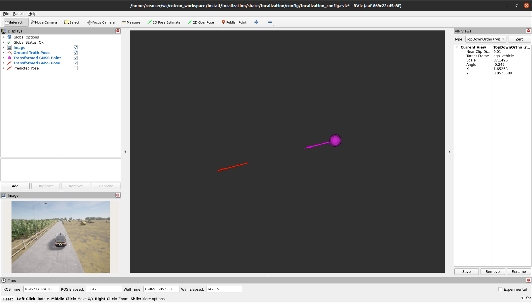
ros2 bag play localization.db3 --clock

If everything is implemented correctly, the output in the RViz window should look like the following:

The red arrow in the RViz 3D-View visualizes the ground truth pose of the vehicle, while the purple sphere shows the corresponding transformed GNSS position of the vehicle. You will quickly notice that the GNSS position is published at a lower frequency compared to the ground-truth position, resulting in the visible position error in the image.

Before we can fuse the lower frequent GNSS measurements with information from odometry in order to obtain a suitable frequency, we first want to estimate a yaw angle from two sequential GNSS positions in Task 4.

Within this task we would like to estimate the vehicle yaw-angle based on two sequential GNSS measurments.

The function you will implement requires two geometry_msgs::msg::PointStamped as input arguments and a geometry_msgs::msg::PoseStamped as output argument. In the ROS 2 geometry_msgs definition, the orientation is given as a quaternion. First, you will calculate the yaw angle based on the two sequential points using trigonometric equations. Afterwards, you will have to convert this into a quaternion using tf2.

Open the GNSSLocalizationNode.cpp at line 147 to implement the desired functionality.

/**
 * @brief This function estimates the yaw-angle of the vehicle with respect to two given point-measurements
 * 
 * @param[in] current_point the current GNSS Point
 * @param[in] last_point the previous GNSS Point
 * @param[out] output_pose geometry_msgs::msg::Pose including the current_point and an additional 2D orientation
 */
void GNSSLocalizationNode::estimateGNSSYawAngle(const geometry_msgs::msg::PointStamped& current_point, const geometry_msgs::msg::PointStamped& last_point, geometry_msgs::msg::PoseStamped& output_pose)
{
    // START TASK 4 CODE HERE
    // calculate the yaw angle from two sequential GNSS-points




    // use header from input point

    // use the position provided through the input point

    // generate a quaternion using the calculated yaw angle



    // END TASK 4 CODE HERE
}

• Use the description in the comment above the function header to implement the corresponding functionality.
• You may use the illustration below to derive the trigonometric equations to calculate the yaw angle
• Use std::atan2 to calculate the arc tangent of $dy/dx$ since it automatically determines the correct quadrant.
• Initialize a tf2::Quaternion object
• The tf2::Quaternion class provides a function setRPY(roll, pitch, yaw) that generates a quaternion from the given roll, pitch and yaw arguments. The function needs to be called on an tf2::Quaternion object
• For roll and pitch use a value of 0
• Since the orientation in a geometry_msgs::msg::PoseStamped message is of type geometry_msgs::msg::Quaternion, we need to convert the tf2::Quaternion object into an geometry_msgs::msg::Quaternion. For this purpose, the tf2_geometry_msgs package offers the tf2::toMsg(q) which requires a tf2::Quaternion as function argument and returns the corresponding geometry_msgs::msg::Quaternion.

Again, we will test the correct implementation by running the compiled ROS 2 node. First, make sure that the implemented code compiles without errors. For this purpose, please run:

# Run from within the colcon_workspace directory
colcon build --packages-up-to localization

After successful compilation, source your workspace

source install/setup.bash

and launch the localization-stack:

ros2 launch localization localization.launch.py

RViz will open but you won't be able to see anything happen. First, we need to play the bag file. Please attach a new terminal to the docker container with ./ros2_run.sh (if you haven't already).

Again, navigate into the colcon_workspace and source the workspace

source install/setup.bash

Navigate into the bag directory and play the bag file:

# Run from within the colcon_workspace directory
cd ../bag
ros2 bag play localization.db3 --clock

If everything is implemented correctly, the output in the RViz window should look like the following:

Again, the red arrow in the RViz 3D-View visualizes the ground truth pose of the vehicle, while the purple sphere shows the corresponding transformed GNSS position of the vehicle. Now, in addition, you will see a purple arrow that indicates the estimated yaw angle of the vehicle.

Finally, we reached the point where we can combine the low-frequent GNSS measurements with the higher-frequent LiDAR-Odometry output.

This step is performed with every incoming LiDAR-Odometry measurement, thus we use the corresponding callback to implement the functionalities.

First of all, in each callback iteration, the current odometry measurement is stored within a local variable current_odometry. Then, it is checked whether a previous odometry measurement is already stored in last_odometry, since we need at least two sequential measurements to derive the incremental movement of the vehicle in between the time of these two measurements.

This incremental movement is derived by the function getIncrementalMovement. At a higher level, this function works as follows. Since the incoming measurements are related to a fixed frame odom defined by the LiDAR odometry node, it is not sufficient to return only the differences of translation and rotation. These differences must be transformed into the vehicle frame associated with the position of the vehicle at the time of the last_odometry_. To derive the incremental movement associated with the pose corresponding to last odometry_, the function internally uses the tf2 functions.

/**
 * @brief This callback is invoked when the subscriber receives an odometry message
 *
 * @param[in] msg input
 */
void GNSSLocalizationNode::odometryCallback(nav_msgs::msg::Odometry::UniquePtr msg)
{
  // store the incoming message in a local object
  nav_msgs::msg::Odometry current_odometry = *msg;
  if(last_odometry_!=nullptr && gnss_map_pose_!=nullptr) // We need at least two odometry measurements and a GNSS estimate
  {
    // derive the incremental movement of the vehicle inbetween two odometry measurements
    geometry_msgs::msg::Vector3 delta_translation;
    tf2::Quaternion delta_rotation;
    if(!getIncrementalMovement(current_odometry, *last_odometry_, delta_translation, delta_rotation)) return;

Now that the incremental movement between two odometry measurements is given, we can define the initial pose that is utilized for predicting the current vehicle pose. The function setInitialPose either sets the variable pose to the latest predicted pose that is stored within the variable predicted_map_pose_, or in case that a new GNSS measurement is available, the function sets pose to this GNSS measurement.

Afterwards, the function posePrediction is responsible to apply the incremental movement onto the initial pose. The content of this function will be implemented by yourself within Task 5.

After the prediction step is performed in posePrediction, the resulting pose estimate is published and stored in the member variable predicted_map_pose_ for usage in the next iteration.

    geometry_msgs::msg::PoseStamped pose;
    // get the initial pose either from GNSS or from the previous iteration
    setInitialPose(pose);
    // predict the corresponding vehicle pose
    posePrediction(pose, delta_translation, delta_rotation);
    // Set timestamp to current odometry stamp
    pose.header.stamp = current_odometry.header.stamp;
    // Save predicted pose for next iteration
    predicted_map_pose_ = std::make_shared<geometry_msgs::msg::PoseStamped>(pose);
    // Publish predicted pose
    publisher_predicted_pose_->publish(*predicted_map_pose_);
  }
  // Save the current odometry as "last_odometry" for next iteration
  last_odometry_ = std::make_shared<nav_msgs::msg::Odometry>(current_odometry);
}

You can now either go on to Task 5 or have a look into the described functions to understand their functionality in more detail.

As described before, the goal of this task is to implement the content of the function posePrediction that is responsible for applying incremental movements onto the initial pose dereived either from a new GNSS measurement or the latest iteration of the prediction step.

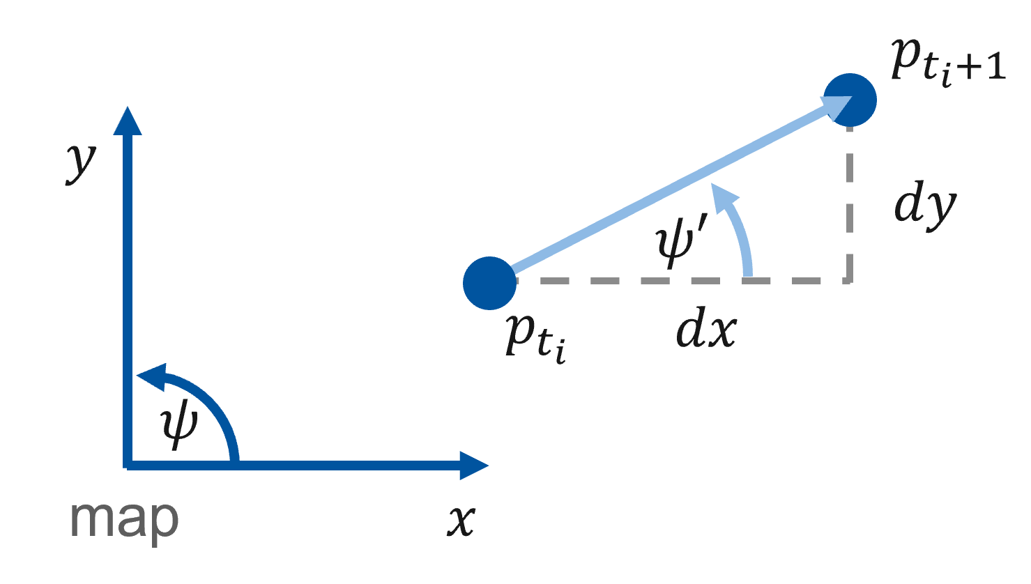
The main implementation task for you is to transform the incremental translations into the map frame. Use the illustration below to solve the task.

Referring to the illustration, $dx'$ and $dy'$ correspond to the variables delta_translation.x and delta_translation.y which are a given input. What we're actually interested in are $dx_{map}$ and $dy_{map}$. We can derive these variables using trigonometric equations. The yaw angle $\psi'$ corresponds to the variable yaw that is provided by the function getYawFromQuaternion (see code below).

To solve the task, perform the following steps:

1. Derive the angle $\alpha$
2. Derive the angle $\beta$
3. Derive $dx_{map}$ and $dy_{map}$
4. Add $dx_{map}$ and $dy_{map}$ to pose.pose.position.x and pose.pose.position.y
5. Apply the delta_rotation to the tf2::Quaternion that represents the orientation of pose given as variable orientation. The multiplication of two quaternions represents two sequential rotations!
6. Use tf2::toMsg to convert the resulting tf2::Quaternion into a geometry_msgs::msg::Quaternion and store this into pose.pose.orientation

Now you're prepared to open the GNSSLocalizationNode.cpp at line 252 to implement the desired functionality.

/**
 * @brief this function performs the actual prediction of the vehicle pose
 * 
 * @param[out] pose the pose on that delta_translation and delta_rotation is applied
 * @param[in] delta_translation the incremental translation of the vehicle (in vehicle coordinates)
 * @param[in] delta_rotation the incremental rotation of the vehicle (in vehicle coordinates)
 */
void GNSSLocalizationNode::posePrediction(geometry_msgs::msg::PoseStamped& pose, const geometry_msgs::msg::Vector3& delta_translation, const tf2::Quaternion& delta_rotation)
{
  // The delta values are given in a vehicle centered frame --> we need to transform them into the map frame
  // First perform the transformation of the translation into map coordinates, by using the yaw of the vehicle in map coordinates
  tf2::Quaternion orientation;
  tf2::fromMsg(pose.pose.orientation, orientation);
  double yaw;
  getYawFromQuaternion(yaw, orientation);
  // START TASK 5 CODE HERE





  // Apply dx and dy (in map coordinates) to the position


  // Last apply delta orientation to the pose
  // the multiplication of two quaternions represents two sequential rotations


  // END TASK 5 CODE HERE
}

• Use the description in the comment above the function header to implement the corresponding functionality.
• You may use the illustration below to derive the trigonometric equations to calculate the translations in the map-frame
• You may use std::atan2, std::sin, std::cos, std::sqrt and std::pow
• The multiplication of two quaternions represents two sequential rotations.

If you finished the implementation of Task 5, you can test the implementation and inspect the final result by running the compiled ROS 2 node. Make sure that the implemented code compiles without errors. For this purpose, please run:

# Run from within the colcon_workspace directory
colcon build --packages-up-to localization

After successful compilation, source your workspace

source install/setup.bash

and launch the localization stack:

ros2 launch localization localization.launch.py

RViz will open, but you won't be able to see anything happen. First, we need to play the bag file. Please attach a new terminal to the docker container with ./ros2_run.sh (if you haven't already).

Again, navigate into the colcon_workspace and source the workspace

source install/setup.bash

Navigate into the bag directory and play the bag file:

# Run from within the colcon_workspace directory
cd ../bag
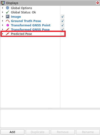
ros2 bag play localization.db3 --clock

In our case, make sure to enable the visualization of the Predicted Pose in the Displays Section of the RViz window by checking the corresponding check box.

If everything is implemented correctly, the output in the RViz window should somehow look like the following:

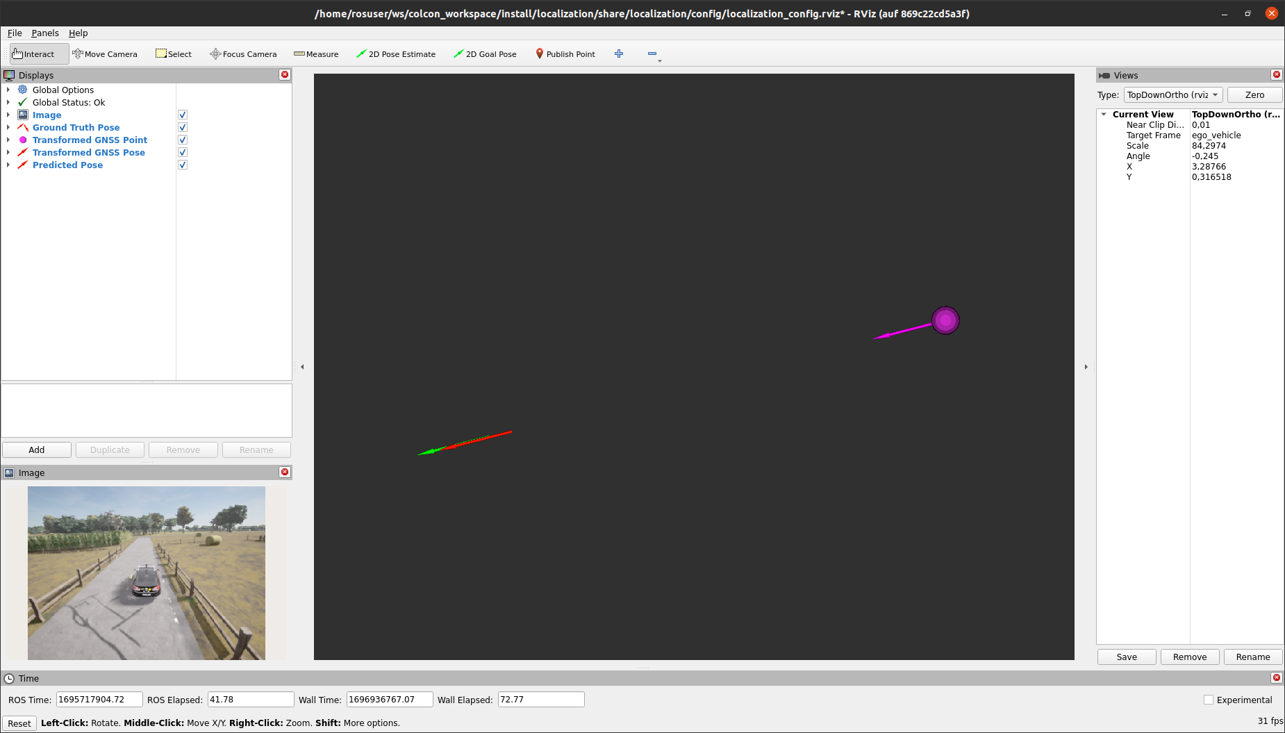
Next to the red (ground truth) and purple arrow (estimated GNSS pose), you will now see a green arrow indicating the predicted pose of the vehicle that results from combining the GNSS estimate with the odometry input.

Congratulations! You have completed the C++ implementation and set up a simple localization stack for automated driving. In the following exercise, we want to evaluate your results in a Jupyter notebook exercise. For this purpose, be sure to record a bag file. The instructions for doing so can be found in the following section.

Make sure that the implemented code compiles without errors. For this purpose, please run:

# Run from within the colcon_workspace directory
colcon build --packages-up-to localization

After successful compilation source your workspace

source install/setup.bash

and launch the localization stack:

ros2 launch localization localization.launch.py

Attach a new terminal to the docker container with ./ros2_run.sh (if you haven't already). Again, navigate into the colcon_workspace and source the workspace

source install/setup.bash

Navigate into the bag directory and start recording a new bag file:

# Run from within the colcon_workspace directory
cd ../bag
ros2 bag record -o localization_evaluation /ground_truth/pose /localization/predicted_pose

Finally, play the bag file. Attach a third terminal to the docker container with ./ros2_run.sh (if you haven't already).

Again, navigate into the colcon_workspace and source the workspace

source install/setup.bash

Navigate into the bag directory and play the bag file:

# Run from within the colcon_workspace directory
cd ../bag
ros2 bag play localization.db3 --clock

After the playback of localization.db3 has finished, cancel the recording of your evaluation bag file by typing ctrl+c in the corresponding terminal.

• You learned how to set up a localization stack for automated driving in an urban environment using ROS 2
• You utilized and investigated KISS-ICP LiDAR Odometry
• You learned how to implement further processing of the lidar odometry output by combining it with low-frequent GNSS measurements
• You learned how to apply projections and transformations to GNSS measurements
• You have completed a simple example for combining GNSS and LiDAR-Odometry measurements for pose estimation of automated vehicles