metaphlan4 - biobakery/biobakery GitHub Wiki
MetaPhlAn is a tool for profiling the composition of microbial communities from metagenomic shotgun sequencing data.
This tutorial has been updated to work with version 4.1.1 and the Oct22 toy database (Made by Franzosa May 28 2025)
- For information about installation and pre-requisites for MetaPhlAn 4.0, please see the manual page.
- Please direct science and software support questions to the MetaPhlAn bioBakery forum topic.
- Legacy tutorials for previous MetaPhlAn versions are also available:
If you're using this tutorial as part of a workshop, or if you'd like to think about the algorithm and implementation details a bit, you'll occasionally see "discussion questions" at the end of tutorial sections, formatted like this:
- What is your quest?
- What is your favorite color?
- 1. Creating taxonomic profiles
- 2. Visualizing taxonomic profiles
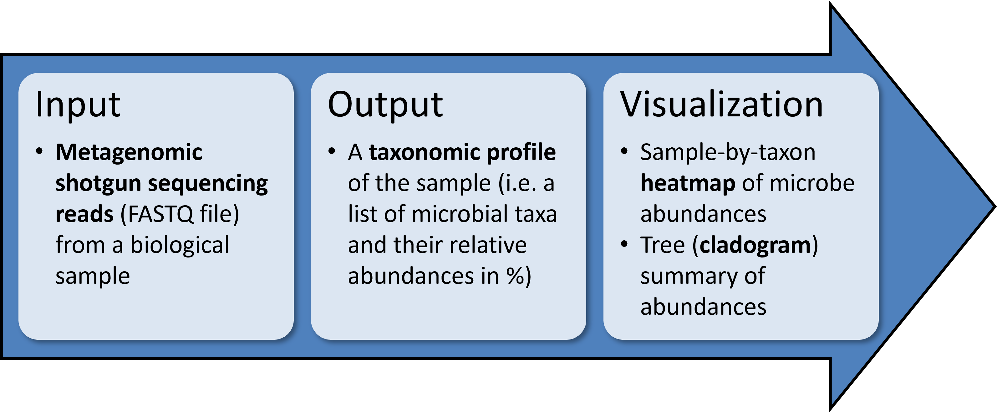
MetaPhlAn accepts as input short reads from a single shotgun metagenomic sequencing experiment and outputs the list of detected microbes and their relative abundances.
MetaPhlAn accepts metagenomic sequence information in several formats, including fastq, fasta, sam, and bowtie2out (a MetaPhlAn-specific mapping summary).
To see all the input formats (and other arguments), type metaphlan -h | less. Use the arrow key to move up and down. Type q to quit back to the command prompt.
usage: metaphlan --input_type {fastq,fasta,bowtie2out,sam} [--force]
[--bowtie2db METAPHLAN_BOWTIE2_DB] [-x INDEX]
[--bt2_ps BowTie2 presets] [--bowtie2_exe BOWTIE2_EXE]
[--bowtie2_build BOWTIE2_BUILD] [--bowtie2out FILE_NAME]
[--min_mapq_val MIN_MAPQ_VAL] [--no_map] [--tmp_dir]
[--tax_lev TAXONOMIC_LEVEL] [--min_cu_len]
[--min_alignment_len] [--add_viruses] [--ignore_eukaryotes]
[--ignore_bacteria] [--ignore_archaea] [--ignore_ksgbs]
[--ignore_usgbs] [--stat_q] [--perc_nonzero]
[--ignore_markers IGNORE_MARKERS] [--avoid_disqm] [--stat]
[-t ANALYSIS TYPE] [--nreads NUMBER_OF_READS]
[--pres_th PRESENCE_THRESHOLD] [--clade] [--min_ab]
[-o output file] [--sample_id_key name]
[--use_group_representative] [--sample_id value]
[-s sam_output_file] [--legacy-output] [--CAMI_format_output]
[--unclassified_estimation] [--mpa3] [--biom biom_output]
[--mdelim mdelim] [--nproc N] [--subsampling SUBSAMPLING]
[--subsampling_seed SUBSAMPLING_SEED] [--install] [--offline]
[--force_download] [--read_min_len READ_MIN_LEN] [-v] [-h]

[INPUT_FILE] [OUTPUT_FILE]

DESCRIPTION: MetaPhlAn version 4.0.2 (22 Sep 2022): [META]genomic [PH]y[L]ogenetic [AN]alysis for metagenomic taxonomic profiling.

AUTHORS: Aitor Blanco-Miguez ([email protected]), Francesco Beghini ([email protected]), Nicola Segata ([email protected]), Duy Tin Truong, Francesco Asnicar ([email protected]).
- Which command line arguments are required?
- Which optional command line arguments seem most important or most commonly used?
For the purpose of this tutorial, we will use the following set of six human metagenomes from the Human Microbiome Project (HMP) which have been downsampled for rapid analysis:
- SRS014476-Supragingival_plaque.fasta.gz
- SRS014494-Posterior_fornix.fasta.gz
- SRS011061-Stool.fasta.gz
- SRS014464-Anterior_nares.fasta.gz
- SRS014470-Tongue_dorsum.fasta.gz
- SRS014472-Buccal_mucosa.fasta.gz
The original files, and many others, can be downloaded from the HMP DACC.
- If you are running this tutorial as a part of short course on a bioBakery cloud instance, the input files have been pre-downloaded. Open a terminal and enter:
    cd Tutorials/metaphlan4
    ls input
- We will create a folder named
metaphlan_analysisalongsideinputandoutputto act as our working directory. - Enter the commands below to create the working directory and copy the input files into it.
    mkdir metaphlan_analysis
    cp input/*.fasta.gz metaphlan_analysis/
- Navigate into the mew
metaphlan analysisfolder and use thelscommand to check if the files have been correctly copied/downloaded.
    cd metaphlan_analysis
    ls
- We are now ready to run MetaPhlAn. Please proceed to the next section of the tutorial.
-
IF you're running this tutorial locally (your PC/laptop), make a new folder in your current working directory with
mkdirand access it withcd. Use this folder for all MetaPhlAn analyses in this tutorial.
    mkdir metaphlan_analysis
    cd metaphlan_analysis
- Click on the links above to download each HMP file. NOTE that if you are using the Google Chrome browser, it may automatically decompress (gunzip) the gzip-ed files. The files should download to your default
Downloads/folder location. Copy the files fromDownloads/to yourmetaphlan_analysis/folder:
cp ~/Downloads/SRS*.fasta.gz .
- Alternatively, you can use the
curlorwgetprograms on MacOS / Linux to download each file directly into the folder you created. Confirm that you are working in themetaphlan_analysis/folder withpwd. Right click on each link, choose "Copy Link Address" (or equivalent), and in a terminal type:
curl -LO $LINK (OR) wget $LINK
-
Where
$LINKis the link you copied to your clipboard. -
Use the
lscommand to verify that the files have been correctly copied/downloaded. Each should be about 700 Kb. We are now ready to run MetaPhlAn.
- If you're familiar with the command line and file structure, does it matter where you place MetaPhlAn's input files, or where you run it from?
- What about these input files might make them particularly appropriate for a short demonstration?
Here is a minimal command for profiling a single metagenome with MetaPhlAn (using the first downsampled HMP file described above as an input):
metaphlan SRS014476-Supragingival_plaque.fasta.gz --input_type fasta > SRS014476-Supragingival_plaque_profile.txt
(NOTE: If this is your first time running MetaPhlAn, the first step in this process involves MetaPhlAn downloading, decompressing, and indexing its marker gene database. This process may take ~30 minutes - depending in part on your download speed - but only needs to be performed once.)
Running MetaPhlAn following the example in the prior section will create two output files. Check what files have been created with ls.
SRS014476-Supragingival_plaque.fasta.gz.bowtie2out.txt
This file contains a reduced representation of the (intermediate) mapping results of your sequencing reads to MetaPhlAn's marker gene sequences. Alignments are listed one-per-line in tab-separated columns of Read ID and Marker Gene ID. Inspect the file by executing:
less -S SRS014476-Supragingival_plaque.fasta.gz.bowtie2out.txt
Which yields:
HWUSI-EAS1568_102539179:1:100:10007:7282/1__1.50        UniRef90_P44049|1__7|SGB9649
HWUSI-EAS1568_102539179:1:100:10008:17064/1__1.53       UniRef90_E0DI50|1__4|SGB17007
HWUSI-EAS1568_102539179:1:100:10012:9508/1__1.85        UniRef90_A0A3S4XT37|1__5|SGB17007
HWUSI-EAS1568_102539179:1:100:10025:5272/1__1.159       UniRef90_A0A3S5F533|1__7|SGB17007
HWUSI-EAS1568_102539179:1:100:10036:1783/1__1.212       UniRef90_A0A2A8D7T0|1__5|SGB49305
HWUSI-EAS1568_102539179:1:100:10075:8243/1__1.442       UniRef90_E0DFG3|1__5|SGB17007
HWUSI-EAS1568_102539179:1:100:10121:4053/1__1.687       UniRef90_E3H4E3|1__10|SGB49305
HWUSI-EAS1568_102539179:1:100:10145:8825/1__1.834       UniRef90_E3H0V0|1__8|SGB49305
HWUSI-EAS1568_102539179:1:100:10147:6525/1__1.845       UniRef90_E0DGM2|1__6|SGB17007
HWUSI-EAS1568_102539179:1:100:10209:16912/1__1.1174     UniRef90_E0DIQ5|1__4|SGB17007
HWUSI-EAS1568_102539179:1:100:10242:17338/1__1.1330     UniRef90_E0DGB7|1__3|SGB17007
HWUSI-EAS1568_102539179:1:100:10250:4528/1__1.1382      UniRef90_A0A269YLE7|1__4|SGB49305
Type q to leave the less interface after inspecting the file.
SRS014476-Supragingival_plaque_profile.txt
This file contains the final computed taxon abundances. Taxon abundances are listed one clade per line, tab-separated from the clade's relative abundance in %:
less -S SRS014476-Supragingival_plaque_profile.txt
Which yields:
[1] # DATABASE VERSION
[2] # COMMAND EXECUTED
[3] # 19048 reads processed
[4] # SampleID Metaphlan_Analysis
[5] # clade_name NCBI_tax_id relative_abundance additional_species
k__Bacteria     2       100.0
k__Bacteria|p__Actinobacteria   2|201174        100.0
k__Bacteria|p__Actinobacteria|c__Actinomycetia  2|201174|1760   100.0
k__Bacteria|p__Actinobacteria|c__Actinomycetia|o__Corynebacteriales     2|201174|1760|85007     55.36506
k__Bacteria|p__Actinobacteria|c__Actinomycetia|o__Micrococcales 2|201174|1760|85006     44.63494
k__Bacteria|p__Actinobacteria|c__Actinomycetia|o__Corynebacteriales|f__Corynebacteriaceae       2|201174|1760|85007|1653        55.36506
...
The file has a five line header (lines beginning with #). We've added [i]s (line numbers) to the header text above to help call out their roles more clearly.
-
[1]: Indicates the version of the marker gene database that MetaPhlAn used in this run. There are currently ~1.1M unique clade-specific marker genes identified from ~100k reference genomes (~99,500 bacterial and archaeal and ~500 eukaryotic) included in the database. -
[2]: Provides a copy of the command that was run to produce this profile. This includes the path to the MetaPhlAn executable, the input file that was analyzed, and any custom parameters that were configured. -
[3]: Indicates the number of sample reads processed. -
[4]: Lists your sample name. -
[5]: Provides column headers from the profile data that follows.
More specifically, [5] includes four headers to be familiar with:
-
clade_name: The taxonomic lineage of the taxon reported on this line, ranging from Kingdom (e.g. Bacteria/Archaea) to species genome bin (SGB). Taxon names are prefixed to help indicate their rank:Kingdom: k__,Phylum: p__,Class: c__,Order: o__,Family: f__,Genus: g__,Species: s__, andSGB: t__. We'll examine these more closely below. -
NCBI_tax_id: The NCBI-equivalent taxon IDs of the named taxa fromclade_name. -
relative_abundance: The taxon's relative abundance in %. Since typical shotgun-sequencing-based taxonomic profile is relative (i.e. it does not provide absolute cell counts), clades are hierarchically summed. Each taxonomic level will sum to 100%. That is, the sum of all kingdom-level clades is 100%, the sum of all phylum-level clades is 100%, and so forth. -
additional_species: Additional species names for cases where the metagenome profile contains clades that represent multiple species. The species listed in column 1 is the representative species in such cases.
Let's use grep to retrieve, format and zoom in on a more specific example, the taxonomic lineage of the first species in the file:
grep s__ SRS014476-Supragingival_plaque_profile.txt | head -1 | cut -f1 | sed 's/|/\n/g'
ℹ️ Command Breakdown and Explanation
This command extracts and formats the full taxonomic lineage of the first species-level entry found in a MetaPhlAn profile output.
grep s__ SRS014476-Supragingival_plaque_profile.txt
- The
grepcommand searches for a pattern (s__) on a text file or command output.- In this case, the command searches for all lines in the profile that include the pattern
s__, which indicates species-level taxonomic entries.- This helps isolate species-resolved taxa like k__Bacteria|p__Firmicutes|...|s__Streptococcus_mutans.
| head -1
- The pipe operator (
|) passes on the output from one command to another.- This means that the
headcommand will run on the result of the previousgrepcommand.headdisplay the first lines (heading lines) of a text stream. It is useful for quick inspection or formatting a small number of lines.- By passing the flag
-1,headwill display only the first line of the text stream.
| cut -f1
- Cuts a tab-delimited line into its corresonding fields.
- The flag
-f1tells the command to retain only the first field after cutting, discarding the rest.- In MetaPhlAn output, the first column typically contains the taxonomic path, while other columns might have abundance values.
| sed 's/|/\n/g'
- This is where the magic happens:
s/|/\n/gis a sed substitution command, broken down as:
s/.../gmeans: perform the substitution...globally (on all matches)|is the character to search for (in MetaPhlAn output, it separates taxonomic ranks)\nis a special escape sequence representing a newline- So: every pipe symbol (
|) in the taxonomy string is replaced with a line break (\n).- Effectively, this transformation prints each rank (kingdom, phylum, class, etc.) on its own line.
This yields the taxonomy of the microbe C. matruchotii:
k__Bacteria
p__Actinobacteria
c__Actinobacteria
o__Corynebacteriales
f__Corynebacteriaceae
g__Corynebacterium
s__Corynebacterium_matruchotii
As an additional experiment, let's verify that the sum of all taxonomic orders' abundances is 100%:
grep o__ SRS014476-Supragingival_plaque_profile.txt | grep -v f__ | cut -f1,3
ℹ️ Command Breakdown and Explanation
_`grep o__` isolates order-resolved lineages while `grep -v f__` removes family-resolved lineages, leaving orders as the most specific taxa; `cut -f 1,3` then isolates the taxonomy column and the relative abundance column._
Which yields:
k__Bacteria|p__Actinobacteria|c__Actinomycetia|o__Corynebacteriales	55.36506
k__Bacteria|p__Actinobacteria|c__Actinomycetia|o__Micrococcales	44.63494
This looks good by visual inspection! We can modify the command above to verify the sum at other taxonomic levels, e.g. species:
grep s__ SRS014476-Supragingival_plaque_profile.txt | grep -v t__ | cut -f1,3 | sed "s/.*|//g"
ℹ️ Command Breakdown and Explanation
This command adds an additional call to
sedto remove the taxonomy up to the species prefix, which helps to make the output a little easier to read.
Which yields:
s__Corynebacterium_matruchotii	55.36506
s__Rothia_SGB49305	44.63494
-
Since the per-clade abundance output file is already normalized, you never need to sum-normalize these relative abundances. However, if you tried to, what would the sum of all clades' relative abundances be?
-
Why do the two species extracted above have the same relative abundances as the two orders extracted with the previous command? (Hint: remove the
sedcommand from the species version to see their full taxonomic lineages.)
When re-analyzing a sample (e.g. using different MetaPhlAn options), it is preferable to start from the sample's .bowtie2out.txt file. This allows you to skip the time-consuming step of mapping the sample's reads to the marker gene database, making the re-analysis much faster.
Let's explore this option by renaming the profile we created above and then regenerating it, this time starting from the .bowtie2out.txt file.
mv SRS014476-Supragingival_plaque_profile.txt SRS014476-Supragingival_plaque_profile_original.txt
Note that we will need to change the --input_type argument from our original command since we are not starting from raw reads:
metaphlan SRS014476-Supragingival_plaque.fasta.gz.bowtie2out.txt --input_type bowtie2out > SRS014476-Supragingival_plaque_profile_regenerated.txt
This command should finish notably faster than the original run (which was already fast). Verify that the regenerated profile matches the one produced directly from the sample's fastq file (e.g. by extracting and examining species-level abundances using the grep commands introduced in the previous section).
MetaPhlAn can take advantage of multiple cores using the nproc flag. Let's profile one of the other HMP samples, again starting from raw reads, this time using 4 cores during the read-mapping stage:
metaphlan SRS011061-Stool.fasta.gz --input_type fasta --nproc 4 > SRS011061-Stool_profile.txt
(Note: nproc is used by bowtie2 which processes 10K reads per second per thread. Since we have a very small number of reads in this demo, the difference in speed up is negligible.)
Each MetaPhlAn execution processes exactly one sample, but the resulting single-sample analyses can easily be combined into an abundance table spanning multiple samples. Let's finish the last four samples from the input files tutorial section:
metaphlan SRS014464-Anterior_nares.fasta.gz --input_type fasta --nproc 4 > SRS014464-Anterior_nares_profile.txt
metaphlan SRS014470-Tongue_dorsum.fasta.gz --input_type fasta --nproc 4 > SRS014470-Tongue_dorsum_profile.txt
metaphlan SRS014472-Buccal_mucosa.fasta.gz --input_type fasta --nproc 4 > SRS014472-Buccal_mucosa_profile.txt
metaphlan SRS014494-Posterior_fornix.fasta.gz --input_type fasta --nproc 4 > SRS014494-Posterior_fornix_profile.txt
Alternatively, if you are familiar with shell syntax, you can loop over all input files (make sure you have deleted previously generated Bowtie 2 output files to prevent errors):
for i in SRS*.fasta.gz; do metaphlan $i --input_type fasta --nproc 4 > ${i%.fasta.gz}_profile.txt; done
Either way, you will now have a complete set of six profile output files and six intermediate mapping files. If you'd like to skip this step to speed things up, the 12 demo file outputs can be downloaded from the following links (right-click on the link and pick "Save Link as..." or click on the link and then right-click on the preview page and select "Save Page as...", or copy the URL to download on a server).
If you are running this tutorial as part of a short course, the Bowtie 2 output files and profile files are in the output/ folder. To copy them to the current directory:
- first, check that you are in the working directory (
metaphlan_analysis):
pwd
- Then, after confirming you ar ein the working directory, clean up the files using
rm *:
rm *
- Finally, copy the precomputed outputs into the current folder
cp ../output/*_profile.txt .
- SRS011061-Stool_profile.txt
- SRS014464-Anterior_nares_profile.txt
- SRS014470-Tongue_dorsum_profile.txt
- SRS014472-Buccal_mucosa_profile.txt
- SRS014476-Supragingival_plaque_profile.txt
- SRS014494-Posterior_fornix_profile.txt
- SRS011061-Stool.fasta.gz.bowtie2out.txt
- SRS014464-Anterior_nares.fasta.gz.bowtie2out.txt
- SRS014470-Tongue_dorsum.fasta.gz.bowtie2out.txt
- SRS014472-Buccal_mucosa.fasta.gz.bowtie2out.txt
- SRS014476-Supragingival_plaque.fasta.gz.bowtie2out.txt
- SRS014494-Posterior_fornix.fasta.gz.bowtie2out.txt
Finally, the MetaPhlAn distribution includes a utility script that will create a single tab-delimited table from a set of sample-specific abundance profiles (isolating the sample names, feature taxonomies, and relative abundances):
merge_metaphlan_tables.py *_profile.txt > merged_abundance_table.txt
You can also download the merged table from here:
This table can be opened as a spreadsheet (using a program like Excel), any gene expression analysis program, less (example below), or visualized graphically as per subsequent tutorial sections:
less -S merged_abundance_table.txt
The first few lines look like:
#toy_vOct22_CHOCOPhlAnSGB_202403
clade_name      SRS011061-Stool SRS014464-Anterior_nares        SRS014470-Tongue_dorsum SRS014472-Buccal_mucosa SRS014476-Supragingival_plaque  SRS014494-Posterior_fornix
k__Bacteria     100.0   100.0   100.0   100.0   100.0   100.0
k__Bacteria|p__Bacteroidetes    91.43203        0.0     23.26112        0.0     0.0     0.0
k__Bacteria|p__Firmicutes       8.56797 0.0     76.73888        83.83307        0.0     100.0
k__Bacteria|p__Bacteroidetes|c__Bacteroidia     91.43203        0.0     23.26112        0.0     0.0     0.0
k__Bacteria|p__Firmicutes|c__Clostridia 8.56797 0.0     0.0     0.0     0.0     0.0
k__Bacteria|p__Bacteroidetes|c__Bacteroidia|o__Bacteroidales    91.43203        0.0     23.26112        0.0     0.0     0.0
k__Bacteria|p__Firmicutes|c__Clostridia|o__Eubacteriales        8.56797 0.0     0.0     0.0     0.0     0.0
k__Bacteria|p__Bacteroidetes|c__Bacteroidia|o__Bacteroidales|f__Bacteroidaceae  70.84222        0.0     0.0     0.0     0.0     0.0
k__Bacteria|p__Bacteroidetes|c__Bacteroidia|o__Bacteroidales|f__Tannerellaceae  17.73698        0.0     0.0     0.0     0.0     0.0
k__Bacteria|p__Firmicutes|c__Clostridia|o__Eubacteriales|f__Oscillospiraceae    8.56797 0.0     0.0     0.0     0.0     0.0
k__Bacteria|p__Bacteroidetes|c__Bacteroidia|o__Bacteroidales|f__Muribaculaceae  2.85283 0.0     0.0     0.0     0.0     0.0
k__Bacteria|p__Bacteroidetes|c__Bacteroidia|o__Bacteroidales|f__Bacteroidaceae|g__Bacteroides   36.91102        0.0     0.0     0.0     0.0     0.0
k__Bacteria|p__Bacteroidetes|c__Bacteroidia|o__Bacteroidales|f__Bacteroidaceae|g__Phocaeicola   33.9312 0.0     0.0     0.0     0.0     0.0
k__Bacteria|p__Bacteroidetes|c__Bacteroidia|o__Bacteroidales|f__Tannerellaceae|g__Parabacteroides       17.73698        0.0     0.0     0.0     0.0     0.0
k__Bacteria|p__Firmicutes|c__Clostridia|o__Eubacteriales|f__Oscillospiraceae|g__Oscillospiraceae_unclassified   8.56797 0.0     0.0     0.0     0.0     0.0
-
In what important ways does analysis of a relative abundance table differ from that of a gene expression (microarray or RNA-seq) transcript table? In what ways are they similar?
-
Under what circumstances is this tab-delimited text data format particularly efficient or inefficient? Is this likely to be a problem for species-level taxonomic profiles?
A heatmap is one way to visualize tabular abundance results such as those from MetaPhlAn. The plotting tool we'll use here, hclust2, is a convenience script that can show any, some, or all of the microbes or samples in a MetaPhlAn table. In this tutorial we will plot the heatmap for all of the samples.
If you're using this tutorial from the bioBakery VM (locally or on the cloud), hclust2 is already installed! Otherwise, you can install hclust2 and other bioBakery tools automatically with Conda. :
conda install -c biobakery hclust2
This will install hclust2 and all of its dependencies.
Run the following command to create a species only abundance table, providing the abundance table (merged_abundance_table.txt) created in prior tutorial steps as the first file argument in the chain:
grep -E "s__|SRS" merged_abundance_table.txt \
| grep -v "t__" \
| sed "s/^.*|//g" \
| sed "s/SRS[0-9]*-//g" \
> merged_abundance_table_species.txt
(Command explained: The initial grep command is isolating the header row, which matches SRS, or any species-resolved row containing s__; the second grep command then excludes rows that are also resolved to the SGB level, matching t__; the first sed command removes everything up to the s__ prefix from the species' taxonomies; the second sed command simplifies the sample names.)
The new abundance table (merged_abundance_table_species.txt) will contain only the species abundances with just the species names as the row headers (instead of their full taxonomy) and just the body site names as the column headers (removing the specific SRS sample numbers).
The first few lines of the file will look like:
clade_name      Stool   Anterior_nares  Tongue_dorsum   Buccal_mucosa   Supragingival_plaque    Posterior_fornix
s__Bacteroides_cellulosilyticus 36.91102        0.0     0.0     0.0     0.0     0.0
s__Phocaeicola_vulgatus 33.9312 0.0     0.0     0.0     0.0     0.0
s__Parabacteroides_merdae       17.73698        0.0     0.0     0.0     0.0     0.0
s__Oscillospiraceae_bacterium   8.56797 0.0     0.0     0.0     0.0     0.0
s__GGB1535_SGB2118      2.85283 0.0     0.0     0.0     0.0     0.0
s__Moraxella_nonliquefaciens    0.0     79.13867        0.0     0.0     0.0     0.0
s__Corynebacterium_pseudodiphtheriticum 0.0     20.86133        0.0     0.0     0.0     0.0
s__Veillonella_dispar   0.0     0.0     76.73888        0.0     0.0     0.0
s__Prevotella_histicola 0.0     0.0     23.26112        0.0     0.0     0.0
s__Streptococcus_mitis  0.0     0.0     0.0     83.83307        0.0     0.0
s__Haemophilus_haemolyticus     0.0     0.0     0.0     16.16693        0.0     0.0
s__Corynebacterium_matruchotii  0.0     0.0     0.0     0.0     55.36506        0.0
s__Rothia_SGB49305      0.0     0.0     0.0     0.0     44.63494        0.0
s__Lactobacillus_crispatus      0.0     0.0     0.0     0.0     0.0     77.36286
s__Lactobacillus_iners  0.0     0.0     0.0     0.0     0.0     21.60871
s__Lactobacillus_jensenii       0.0     0.0     0.0     0.0     0.0     1.02844
- Why is it useful to visualize (and particularly to cluster) only the "tips" of the taxonomic tree?
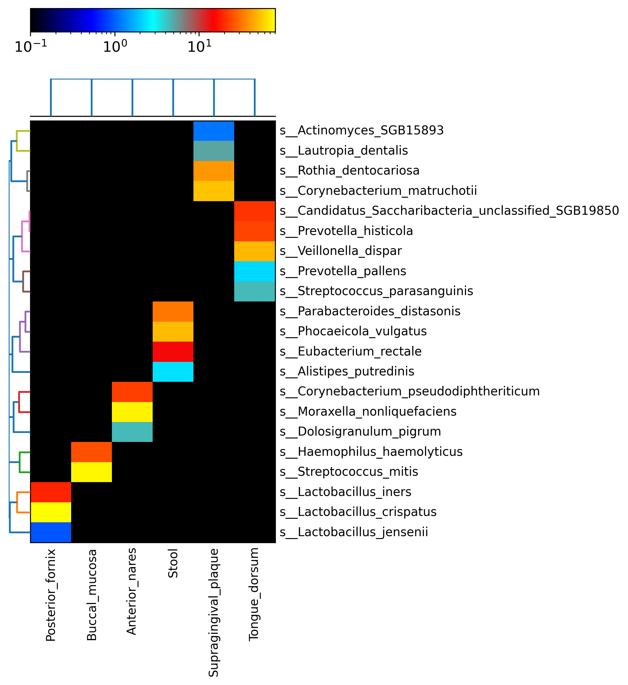
Next generate the species only heatmap by running the following command:
hclust2.py \
-i merged_abundance_table_species.txt \
-o metaphlan4_abundance_heatmap_species.png \
--f_dist_f braycurtis \
--s_dist_f braycurtis \
--cell_aspect_ratio 0.5 \
--log_scale \
--flabel_size 10 --slabel_size 10 \
--max_flabel_len 100 --max_slabel_len 100 \
--minv 0.1 \
--dpi 300
We have only 16 microbes in this demo file but typically, for ease of viewing, one can show the top 25 species using the --ftop 25 argument. This command:
- uses Bray-Curtis as the distance measure both between samples (s) and between features (f) (i.e. species);
- sets the ratio between the width/height of cells to 0.5
- uses a log scale for assigning heatmap colors
- sets the sample and feature label size to 10
- sets the max sample and feature label length to 100
- selects the minimum value to display as 0.1, and
- selects an image resolution of 300 (in that order!).
You can learn more about these options by executing hclust2.py --help.
Open the resulting heatmap (metaphlan4_abundance_heatmap_species.png) to take a look. If you generated it on your local computer, just double click. If you're using a server with just a terminal interface, you might have to transfer the file locally first using a tool like scp. If you're using a server with a graphical interface, you can open the file using a command like see metaphlan4_abundance_heatmap_species.png. Using any of these methods, the results should look like:

Notice that due to the very large differences between body site communities in the human microbiome, we can still easily see site-specific species despite the small demonstration input files (each is subsampled to only 10,000 reads for efficiency).
- Which microbes are most abundant at each body site in these demonstration data?
- Under what circumstances is log-scaling the heatmap abundance colors good? When might it be bad (i.e. visually deceptive)?