Displaying character states on a tree - arklumpus/TreeViewer GitHub Wiki
This guide will provide instructions on how to draw a phylogenetic tree displaying character states together with the tree topology.
The tree file Bacteria.tre contains a rooted tree with 166 bacterial strains. The tree was created mainly based on the NCBI taxonomy, so the topology might not be particularly accurate; this is OK for this example, because we are only interesting in showing the distribution of some features in the tree, without the pretense of providing an accurate bacterial tree of life. The root of the tree is also placed rather arbitrarily.
When the tree file is opened in TreeViewer, it should look similar to the following figure:

The tree is rather hard to read, owing to the many strains and the different branch lengths. To improve it and make it easier to read, we can first of all transform the branch lengths, so that the tree looks more like a cladogram.
To do this, open the modules panel by clicking on the Further transformations button in the Modules tab and click on the Add module button to add a new Transform lengths module. This module can be used to make all the branch lengths in the tree equal to each other, or to transform the tree into a cladogram. To transform the tree in a cladogram, expand the options for the Transform lengths module and set the Transform parameter to Cladogram.
At this point, the branch length labels are not particularly useful and can be removed from the plot by clicking on the Plot actions button in the Modules tab and then on the × button next to the second Labels module in the Plot elements. The tip labels can also be removed, since with so many taxa the tree would be very hard to read anyways.
To increase the vertical spacing between the branches of the tree, click on the Coordinates module button in the Modules tab, then expand the parameters of the module and set the Height to 4000. Finally, you can make the branches thicker and easier to see by expanding the options of the Branches module in the plot elements section and setting the Line weight to 5.
The tree should now look similar to the following image:

A tree file only contains the phylogenetic relationships between the various taxa, and does not include information about additional character state data. This information can be included by adding an "Attachment" to the tree. The file Bacteria_data.tsv contains a table that specifies, for each bacterial strain in the tree:
-
The kind of photosynthetic reaction centre that the bacterium has; this character has 4 possible states:
-
N, if the bacterium does not have any photosynthetic reaction centre genes. -
A, if the bacterium has genes for a Type I reaction centre. -
B, if the bacterium has genes for a Type II reaction centre. -
C, if the bacterium has genes for both Type I and Type II reaction centres (i.e. cyanobacteria).
-
-
The presence or absence of a norV nitric oxide reductase gene:
-
Yif this gene is present. -
Nif this gene is absent.
-
-
The presence or absence of the hmpA gene (which is another gene involved in nitric oxide detoxification):
-
Yif this gene is present. -
Nif this gene is absent.
-
-
A colour in RGB hex format (based on the group to which the bacterium belongs).
-
The group to which the bacterium belongs.
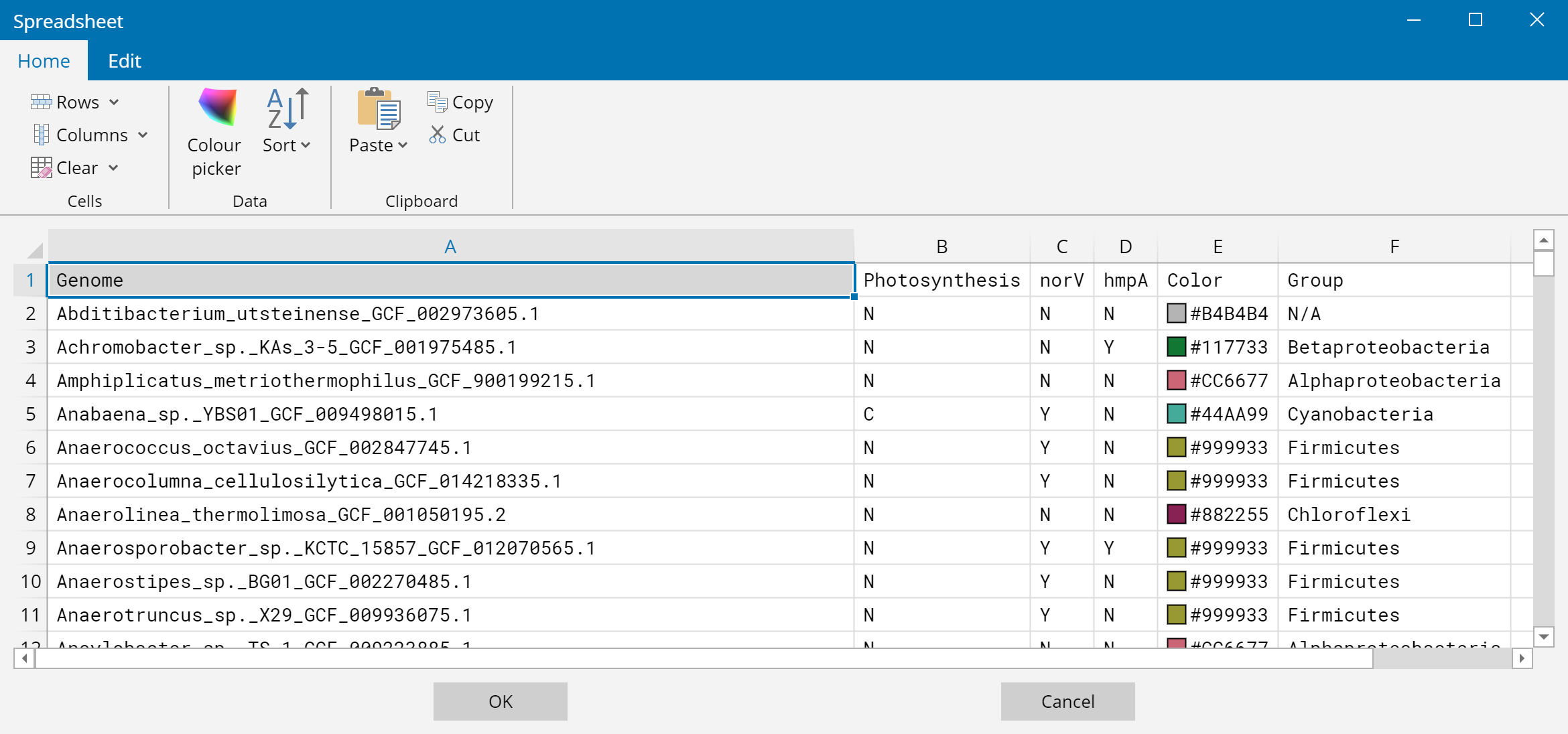
If you open the file in a text editor, you will see that it looks similar to this:
Genome                                          Photosynthesis    norV    hmpA    Color     Group
Abditibacterium_utsteinense_GCF_002973605.1           N            N       N     #B4B4B4    N/A
Achromobacter_sp._KAs_3-5_GCF_001975485.1             N            N       Y     #117733    Betaproteobacteria
Amphiplicatus_metriothermophilus_GCF_900199215.1      N            N       N     #CC6677    Alphaproteobacteria
Anabaena_sp._YBS01_GCF_009498015.1                    C            Y       N     #44AA99    Cyanobacteria
Anaerococcus_octavius_GCF_002847745.1                 N            Y       N     #999933    Firmicutes
Anaerocolumna_cellulosilytica_GCF_014218335.1         N            Y       N     #999933    Firmicutes
Anaerolinea_thermolimosa_GCF_001050195.2              N            N       N     #882255    Chloroflexi
...
This file can be added as an attachment to the TreeViewer plot by clicking on the Add attachment button in the Attachments tab. After selecting the file, click OK on the dialog window that opens to load the Attachment with the default settings. The attachment is shown as a paperclip in the Attachments tab; by clicking on the paperclip you can perform various actions (such as deleting the attachment or exporting it in order to recreate the original file). Note that once a file is added as an attachment to the tree, it becomes completely independent of the original file on your computer. One of the actions you can do by clicking on the paperclip button is to select the Spreadsheet editor option: this will open the attachment in a spreadsheet interface, which can be useful to make quick changes to the file within TreeViewer. In cells that contain a colour (like the Color column), a small square shows a colour preview; you can double-click on these to open a colour picker that lets you easily change the colour.
After adding the file to the plot, we need to tell TreeViewer how to interpret the data contained in it and associate it to the tips of the tree. This can be done by adding a new Parse node states module to the Further transformations. Once the module has been added, expand the options for this module and select the Bacteria_data attachment as the Data file, then check the Use first row as header check box in the New attribute section. This parameter tells TreeViewer to use the first row of the file to determine the column headers. If you click on the Preview button, you will get a preview of the data that will be parsed from the file (so that you can check that everything is in order).
Finally, click on the Apply button to add the attributes to the tree. Now, if you click on any leaf of the tree and open the attributes section of the selection panel, you will see the new attributes Photosynthesis, norV, hmpA, Color and Group that have been loaded from the file. The colour of the terminal branches will also change to reflect the colour contained in the data file.
The tree should now look similar to the following figure:

Currently, all internal branches in the tree are black, even those within coloured groups. To ensure that these internal branches also take the colour of the group they belong to, we can use the Propagate attribute module. Add the module to the Further transformations by clicking on the Add module button, then expand its options and set the Attribute to Color and the Attribute type to String. Now, set the Default value to #B4B4B4 (i.e. the same grey that is specified in the file for strains that do not belong to any of the highlighted groups). You can then click on the Apply button to update the tree.
This module traverses the tree from the tips towards the root; at each node, it checks whether all the children have the same value for the specified attribute (in this case, Color): if they do (which is the case e.g. for two strains in the same group), it applies the same value to the ancestor node as well. If they have different values, it does not propagate the attribute further, and uses the specified Default value instead.
We can now plot the actual character state data on the tree. To do so, you need to use a Node states Plot action module, which can be added to the tree by clicking on the Add module button in the Plot elements section. By default, the node states will be drawn as circles on the tips of the tree (you may want to zoom in to see them better).
To set up the way that the node states are displayed, open the options for the module and, first of all, set the Attribute (at the bottom) to Photosynthesis. This will update the plot, so that the circles reflect the kind of photosynthetic reaction centre each strain has. To change the colour associated with each reaction centre type, click on the Wizard edit state colours button. This will open a new window, in which you can specify the colour for the A, B, C, and N states. For example, you can set the following colours:
- For the
Astate (i.e. Type I reaction centres), a dark orange colour (#D55E00). - For the
Bstate (i.e. Type II reaction centres), a light blue colour (#56B4E9). - For the
Cstate (i.e. cyanobacterial Photosystems I and II), a green colour (#009E73). - For the
Nstate (i.e. non-photosynthetic strains), a grey colour (#DCDCDC).
We now need to position the character state plots appropriately. To move them to the right of the tree labels, you can set the X component of the Position to 50. We can also change the plot Type to Rectangle and increase the Width and Height to 50 and 27, respectively. This will make it easier to see the state associated to each strain.
The plot should now look similar to the following figure:

We can add information about the other character states (i.e. the presence or absence of hmpA and norV) by adding more instances of the Node states Plot action module.
To show the data for norV, after adding the new Node states module, set the Attribute to norV, the X component of the Position to 120, the plot Type to Rectangle, the Width to 50 and the Height to 27. Finally, click on the Wizard edit state colours button and set the colour for the Y state (i.e. presence of the gene) to a red-pink hue (
#CC79A7) and the colour for the N state (i.e. absence of the gene) to grey (
#DCDCDC).
Similarly, for the hmpA gene, set the Attribute to hmpA, the X component of the Position to 190, the plot Type to Rectangle, the Width to 50 and the Height to 27. In this case, we can use an orange colour (
#E69F00) for the Y state, and the same grey colour for the N state (
#DCDCDC).
The tree should now look similar to the following image:

Right now, while the various groups of bacteria have different colours, the tree does not show their names. To make the tree easier to interpret, we can show the group names.
In order to do this, first of all we need to propagate the Group attribute the same way that we propagated the Color attribute: add another instance of the Propagate attribute module to the Further transformations, and set the Attribute to Group, the Attribute type to String and then delete the Default value (so that the text box is empty). Then, click on the Apply button.
Now, you can add a Group labels Plot action module to the tree plot. In the options for this module, set the Attribute to Group and make sure that the Only on last ancestor check box is checked (otherwise, a separate label will be shown for each strain). You should notice that the labels are currently drawn on the left side of the tree (near the root). To move them to the right, you should increase the Distance parameter to 2520.
The text of the labels is a bit too small; to adjust this, you should change the Height to 100, and then click on the Font button to increase the font size to 75. The labels should now become larger and more visible. You will notice that the program does its best to prevent the labels from overlapping on each other. To increase the spacing between the "rows" of labels, increase the Row margin to 25.
As you can see, there are multiple labels that read N/A: this is because, in the data file, strains that do not belong to any of the groups that are highlighted on the tree had this value in the Group column. To prevent these labels from showing up on the tree, we can "delete" them by replacing the N/A values with empty strings. There are multiple ways to do this. For example, if you click on the Search button in the Actions tab, a search bar will appear. Now, if you click on Advanced to open the advanced search options, you can select Group as the Attribute to search. Then, enter N/A in the Search box and leave the Replace with box empty (notice how all the strains that match the criterion have become highlighted). Finally, click on the Replace all button. This will add a new instance of the Replace attribute module to the Further transformations that performs the required substitution. The N/A labels should now disappear.
The tree should now look similar to the following figure:

The final touch that is missing is a legend to identify the meaning of the various colours for the tip states. This can be added using the Legend module.
To add a legend, add a new Plot action module, and select the Legend module. A legend will appear at the bottom of the tree, with a red circle, a blue square and a green star. Expand the options of this module, and click on the Edit button for the Markdown source parameter. In the Markdown editor window, enter the following Markdown code:
### **Legend**
**Photosynthesis** \
 Non-photosynthetic taxon \
 Type I reaction centre \
 Type II reaction centre \
 Photosystems I and II
**_norV_ Gene** \
 Absent \
 Present
**_hmpA_ Gene** \
 Absent \
 PresentSee the readme for the Legend module for more information about the "special image" syntax used to draw the coloured squares.
We now need to position the legend appropriately and to increase the font size. To align the top-left corner of the legend with the top-left corner of the tree plot, set both the Anchor and Alignment to Top-left. Then, increase the Width of the legend to 1000 and the Font size to 70. Finally, to prevent the legend from hiding the branches of the tree, you can change the Background colour to a completely transparent colour (or, alternatively, drag the Legend module up until it appears in the Plot elements list before the Branches).
The final tree figure should be similar to the following:

You can now save the tree file or the plot as a PDF or SVG file using the items from the File menu. You can also download the Bacteria.tbi tree file, which contains the tree along with all the modules.
A plot like this makes it easy to see to identify the character states for the various groups in the tree, as well as to highlight the [lack of] co-occurrence of different features (e.g., from this tree it can be easily seen that most strains with the hmpA gene do not have the norV gene and vice versa).
If you do not like the vertical layout (or the fact that the text for the group labels is rotated), you can rotate the tree by expanding the options for the Coordinates module and setting the Rotation to e.g. 270° using the button. Then, you just need to reposition the legend by changing its Anchor and Alignment to Bottom-left and setting the Y component of the Position to 300 (you can of course specify a different position, if you wish). The rest of the plot will be updated automatically to fit the new layout! The figure will look similar to the following:

This kind of plot is also particularly appropriate for being displayed as a circular tree. To change the layout to a circular tree, do not click on the Circular style button (because this will reset the plot elements that we have spent so much time customising to the default). Instead, click on the Reshape tree button and select Circular style from the drop-down menu. This will update the plot settings without removing our customisations. Then expand the options for the Coordinates module and set the Outer radius to 1500, then click on Apply.
Then, open the options for each Node states module and set the Anchor to Origin. Increase the X component of the position for each module (e.g. set it to 1550 for the first module, 1620 for the second module and 1690 for the third module). Now, set the plot Type to Wedge and update the Width so that it is equal to the Suggested width. You can also increase the Height to 50 for all three modules.
In the options for the Group labels module, reduce the distance to e.g. 1750. You can also click on the Font button and increase the font size to 100.
Finally, reposition the legend by changing its Anchor to Middle-right and the Alignment to Middle-left and set the Position so that the X is equal to 500 and the Y is set at 0. The new plot should look similar to this figure:

The Bacteria_circular.tbi tree file contains the circular tree plot with all the modules. The finished tree file is also available in the Examples section of TreeViewer's welcome page in the File page.