4.5.1 In unity, strength... - Valdes-Tresanco-MS/AMDock-win GitHub Wiki
Sometimes, after performing a molecular docking we observe two poses completely different but with almost the same score. So, what should we do in that case?
There are several alternatives you can use for discarding one of the poses:
- Based on experimental results (mutagenesis, NMR, the crystal structure of similar ligands, etc)
- Using MD simulations and Free Energy Calculations (See Hernández-González et al.)
- Using an "orthogonal" docking engine (with a different searching algorithm and scoring function)
Due to its importance, we are going to use as a case study the SARS-CoV-2 main protease bound to potent broad-spectrum non-covalent inhibitor X77. The structure of the complex was resolved recently (PDB ID: 6W63). Let's see if we can reproduce the pose in the crystal structure by using molecular docking. As we are performing a standard re-docking experiment, the ligand coordinates should be extracted from the complex and randomized.
Receptor (6w63.pdb) and ligand (ligand.pdb) files are available at Installation_path/Doc/Tutorials/V_Additional_Tutorials/1.In_unity_strength folder. The crystal structure of the complex (complex.pdb) is available as well for comparison purposes.
Let's try first with Vina:
- Open AMDock program
- Select Autodock Vina
- Set the Project Name (default Docking_Project)
- Set the Location for Project and push the button “Create Project”
- Check that “Simple Docking” checkbox is selected (It is checked by default)
- Choose the receptor file(Installation_path/Doc/Tutorials/V_Additional_Tutorials/1.In_unity_strength/6w63.pdb)
- Choose the ligand file (Installation_path/Doc/Tutorials/V_Additional_Tutorials/1.In_unity_strength/ligand.pdb)
- Press the “Prepare Input” button
- Then, for defining a search space, pick “Center on Hetero” and select the ligand “A:X77:401”
- Press “Define Search Space” button
Once the search space is defined, you can see the box in the receptor by pressing the button “Show in PyMOL”

- Press the “Run” button
- When docking run ends, the “Results Analysis” tab will appear automatically. There, you will observe a summarizing table with Binding Energies, Estimated Ki values, and Ligand Efficiencies.
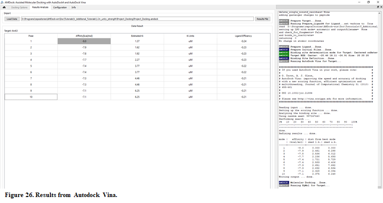
The number of poses and energies can vary since this is docking engine dependent. But, if you perform a number of docking runs with different random seeds every time, you will see the first two poses getting similar score every time, although they are structurally different
-
In the results table, select the first two poses. Press the button “Show in PyMOL” in the bottom left corner to visualize the complex.
-
The crystal structure can be superposed on the predicted structures. Press “Open” in the upper left corner in PyMOL and find the X-ray structure (Installation_path/Doc/Tutorials/V_Additional_Tutorials/1.In_unity_strength/complex.pdb)
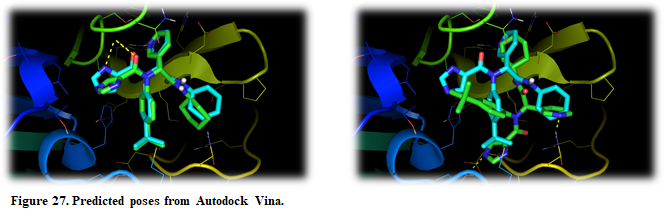
As you can see, both predicted poses are quite different and they possess almost the same score. One of them agrees with the experimental one, but with such a tiny difference in score is risky to sure anything about the predicted poses. In this case, is recommended to try another docking engine, preferably with a different searching algorithm and scoring function. Autodock4 is just what we are looking for! The Atodock4 scoring function is force-field based and it uses LGA for searching.
Let's try now with Autodock4:
- Open AMDock program
- Select Autodock4
- Set the Project Name (default Docking_Project)
- Set the Location for Project and push the button “Create Project”
- Check that “Simple Docking” checkbox is selected (It is checked by default)
- Choose the receptor file(Installation_path/Doc/Tutorials/V_Additional_Tutorials/1.In_unity_strength/6w63.pdb)
- Choose the ligand file (Installation_path/Doc/Tutorials/V_Additional_Tutorials/1.In_unity_strength/ligand.pdb)
- Press the “Prepare Input” button
- Then, for defining a search space, pick “Center on Hetero” and select the ligand “A:X77:401”
- Press “Define Search Space” button
- Press the “Run” button
- When docking run ends, the “Results Analysis” tab will appear automatically. There, you will observe a summarizing table with Binding Energies, Estimated Ki values, and Ligand Efficiencies.

The number of poses and energies can vary since this is docking engine dependent.
-
In the results table, select the first two poses. Press the button “Show in PyMOL” in the bottom left corner to visualize the complex.
-
The crystal structure can be superposed on the predicted structures. Press “Open” in the upper left corner in PyMOL and find the X-ray structure (Installation_path/Doc/Tutorials/V_Additional_Tutorials/1.In_unity_strength/complex.pdb)

In this case, we obtained the same results but this time with a higher difference in scoring between the two first poses. Now that we saw both docking engines predicted the same, it's safer to make conclusions from the predicted poses.