4.2.3 Centered on residue(s) using AutoDock Vina - Valdes-Tresanco-MS/AMDock-win GitHub Wiki
This option is recommended when residues belonging to the binding site are known. This information usually comes from mutagenesis experiments or comparing protein belonging to the same family.
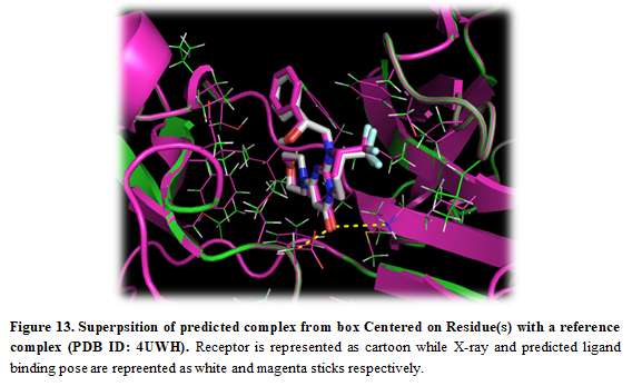
Receptor (4uwh.pdb) and ligand (ligand.pdb) files are available at Installation_path/Doc/Tutorials/I_Simple_Docking/3.Box_Residues folder. The crystal structure of the complex (complex.pdb) is available as well for comparison purposes.
- Open AMDock program or Create a new project in “Results Analysis”
- Select Autodock Vina
- Set the Project Name (default Docking_Project)
- Set the Location for Project and push the button "Create Project"
- Check that “Simple Docking” checkbox is selected (It is checked by default)
- Choose the receptor file (Installation_path/Doc/Tutorials/I_Simple_Docking/3.Box_Residues/4uwh.pdb)
- Choose the ligand file (Installation_path/Doc/Tutorials/I_Simple_Docking/3.Box_Residues/ligand.pdb)
Before going to the next step, go to the configuration tab and check “Ligand Protonation” with OpenBabel.
- Press the “Prepare Input” button
- Then, for defining a search space, pick “Center on Residue(s)”. A text box will appear where residues should be specified by following this notation:
CHAIN:RESIDUE1:NUMBER; CHAIN:RESIDUE2:NUMBER…
AMDock checks automatically if those residues exist in the receptor.
In this tutorial, the following residues were chosen:
A:ILE:634; A:TYR:670; A:PHE:684; A:PHE:758; A:ILE:760
- Press “Define Search Space” button
Once the search space is defined, you can see the box by pressing the button “Show in PyMOL”. In this case, the receptor is represented as cartoon, binding site residues in sticks and the object generated in AutoLigand as mesh representation.

Note: If you want to modify the box, you can use the AMDdock plugin in PyMOL. More details about this procedure here.
- Press the “Run” button
- When docking run ends, the “Results Analysis” tab will appear automatically. There, you will observe a summarizing table with Binding Energies, Estimated Ki values, and Ligand Efficiencies.
The number of poses and energies can vary since this is docking engine dependent.
- In the results table, just the first pose is selected. Press the button “Show in PyMOL” in the bottom left corner to visualize the complex.
If you want to see all the predicted poses, just select all the poses in the result table and press “Show in PyMOL”.
- The crystal structure can be superposed on the predicted structure. Press “Open” in the upper left corner in PyMOL and find the X-ray structure (Installation_path/Doc/Tutorials/I_Simple_Docking/3.Box_Residues/complex.pdb)
- A detailed report of the entire process can be seen on the right side of the screen, which allows for tracking all the results from different programs and algorithms. This log file can be saved in case an error occurred and sent to the developers.