Week 9 (W1 Jan18) Crimes in the UK

Note: For unknown abbreviations and terms, please consider the glossary. If anything is missing, just create an issue or write us an email and we will add it. A list of our data attributes can be found here.

Content

1. Geographical Granularity
2. Feature Selection
3. Next steps

---

Geographical Granularity

As we have written in Week 07 (W51 Dec28) Crimes in the UK, we want to examine the connection between the demographic structure of an area and the number of crimes. Thereby, there area a lot of possibilities to divide UK in areas. Some area types are described in Week 03 (W48 Nov30) Crimes in the UK, furthermore we have also experimented with "Local Authory Areas" during the last weeks and months. Each of the granularities have certainly some advantages; for example, we wanted to use postcode areas at the beginning of the lab, because it is a well known area type, and it is easy to find out which postcode a certain location has.

As preparation to predict the number of crimes in such an area, we have firstly computed the attributes using the datasets we already had:

• Number of crimes broken down to the crime types
• Number of stop and searches in total as well as for each ethnicity, age range and outcome
• Number of point of interests in tatal as well as for 36 categories

For the computation, we have downloaded the boundaries of the areas (MSOA, LSOA) from the Open Geography Portal and performed the calculations using PostGIS.

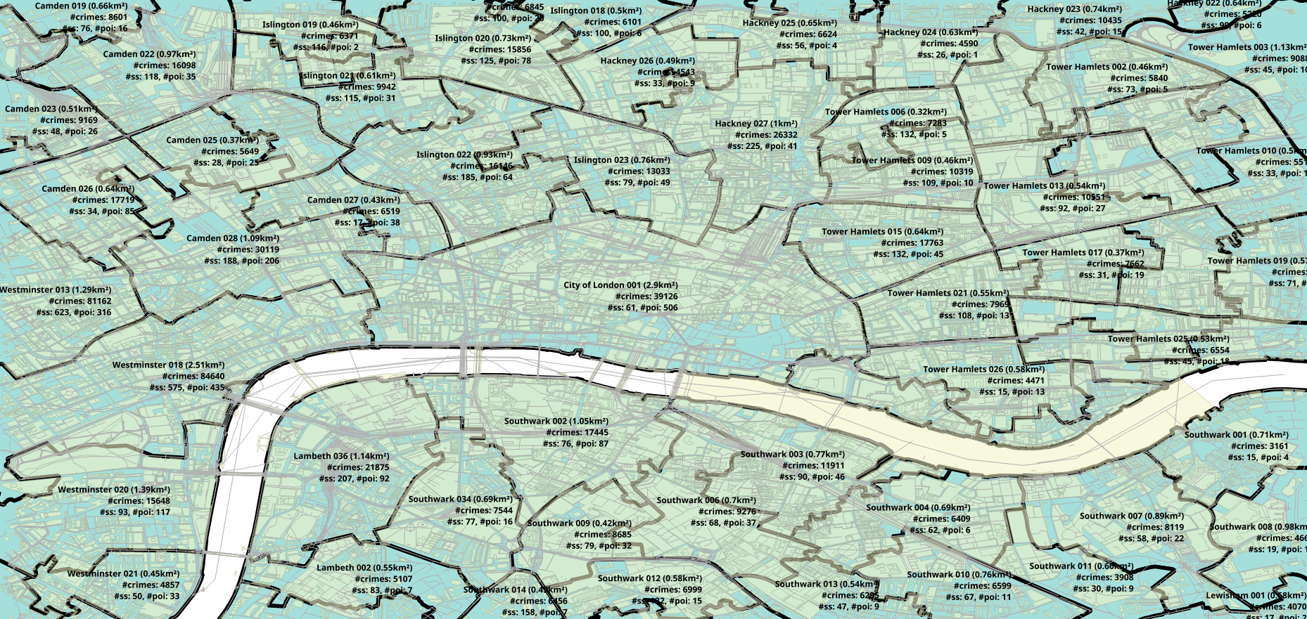
A MSOA has an average size of 21km² and a LSOA an average size of 4km². Here is a map of the centrum of London where the border of MSOAs are black: (Open the images in a new tab to see them in a larger size!)

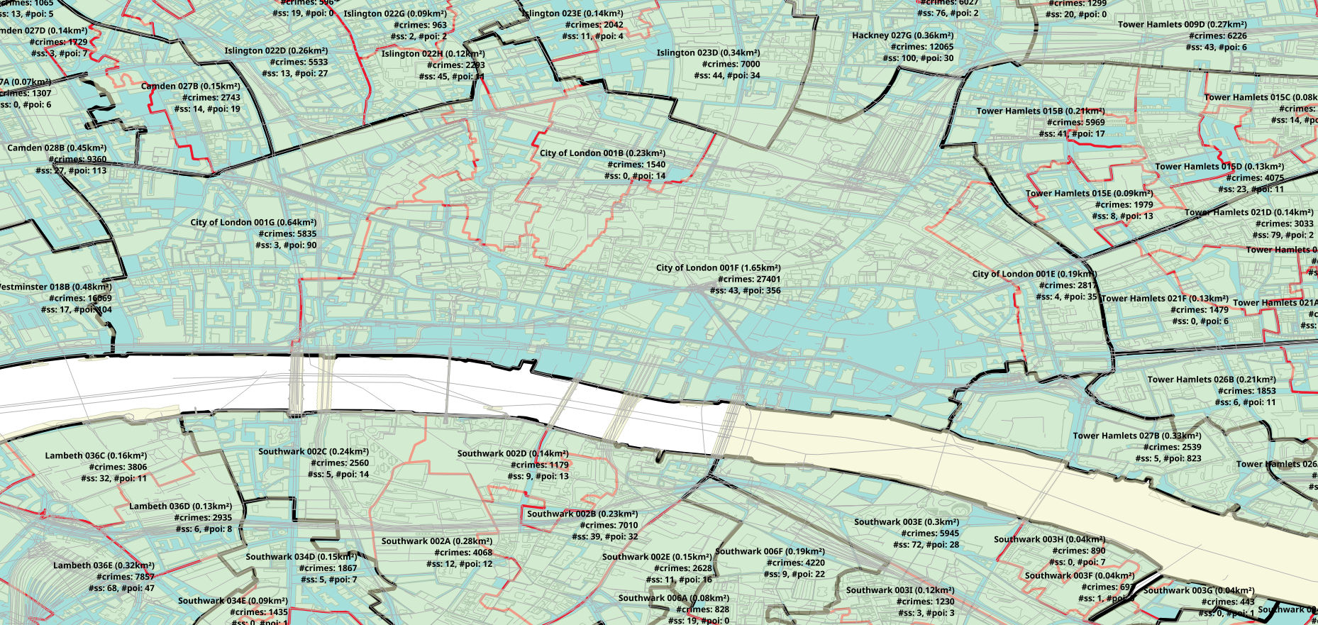
Here are the LSOA borders (red borders):

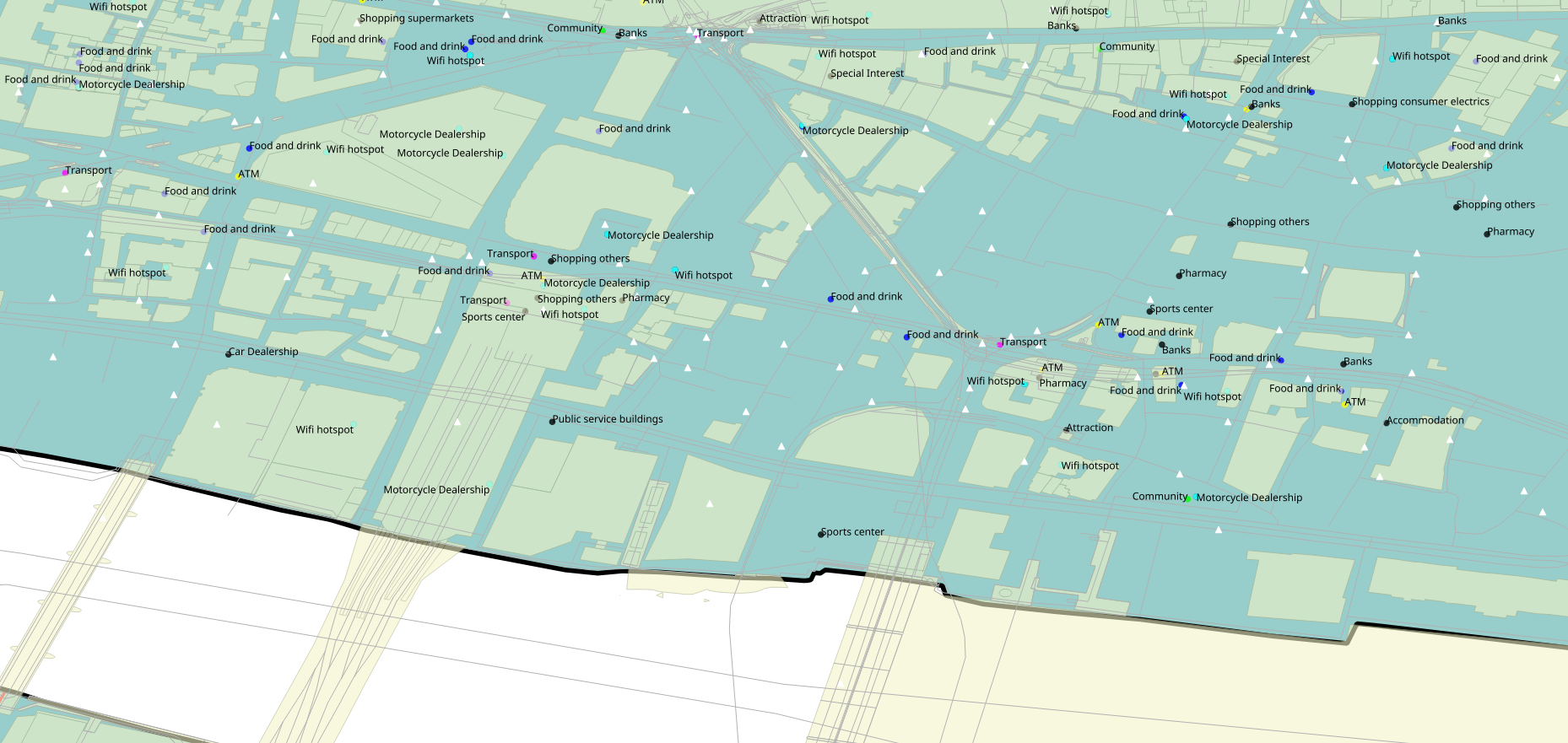
In the following map, the points of interests are displayed as circles. The white triangles are locations, where a crime was marked:

Feature Selection

Last week we automatically parsed all the LSOA and MSOA data that was available from the census 2011. After merging the downloaded files we had 130244 features for each MSOA.

We prepared the data for our first prediction goal. Thus, we did a feature selection where we have chosen the 150 most relevant features for predicting the number of crimes. For this, we used the python libary "scikit learn". The feature selection we did is based on univariate statistical tests. We used the mutual_info_regression function that relies on nonparametric methods based on entropy estimation from k-nearest neighbors distances. Now, we have 150 Features, sorted by relevance, which we will use for the first prediction goal. The features can be found here.

Difficulties

The same as the "Google's N Grams" team, we were not able to use the server. The server always killed our process. However, we used our own powers and created a monster VM in Microsoft Azure that we used to compute the feature selection. It took 340 minutes, with an average RAM usage of 33Gb, to compute the feature selection.

Next steps

• Testing different algorithms on the dataset that we prepared this week for the first prediction goal.
• Afterwards, we will compare the different algorithms and choose a winner.
• Start working on the next prediction goals.

Link to our presentation