Week 03 (W48 Nov30) Crimes in the UK

Note: For unknown abbreviations and terms, please consider the glossary. If anything is missing, just create an issue or write us an email and we will add it.

Content

1. Geographical Inspection
2. First Approach for Predicting Crime Outcome Types
3. Communication with UK Police

---

Geographical Inspection

Up to now, in addition to the coordinates, we also had the Lower Layer Super Output Areas (LSOA) code of the area where a crime happened. LSOAs have an average population size of around 1.500 citizens. This low granularity was i) too small to be visualized on a map in an informative manner ii) not enough to discover location-based patterns. Therefore, we integrated [more geographical data] (https://data.gov.uk/dataset/national-statistics-postcode-lookup-uk/resource/3206f3b9-854a-46ec-8fd2-a6823e836b65). This allowed us to come up with the following geographical structure and therefore derive new features about the crime locations:

Area Type	Description
Latitude/Longitude	The anonymised coordinates. (~800.000 values)
Lower Layer Super Output Area (LSOA)	Small areas defined by the Office for National Statistics with about 1,500 citizens. (~35,000 values)
Middle Layer Super Output Areas (MSOA)	Like LSOA but with about 7,200 citizens. (~7,200 values)
Postcode Area	There are 121 postcode areas in the UK. We have data about crimes in 105 areas.
Region	England can be divided into 9 regions (Wikipedia). Furthermore, we also consider Wales, Scotland and Northern Ireland as regions.

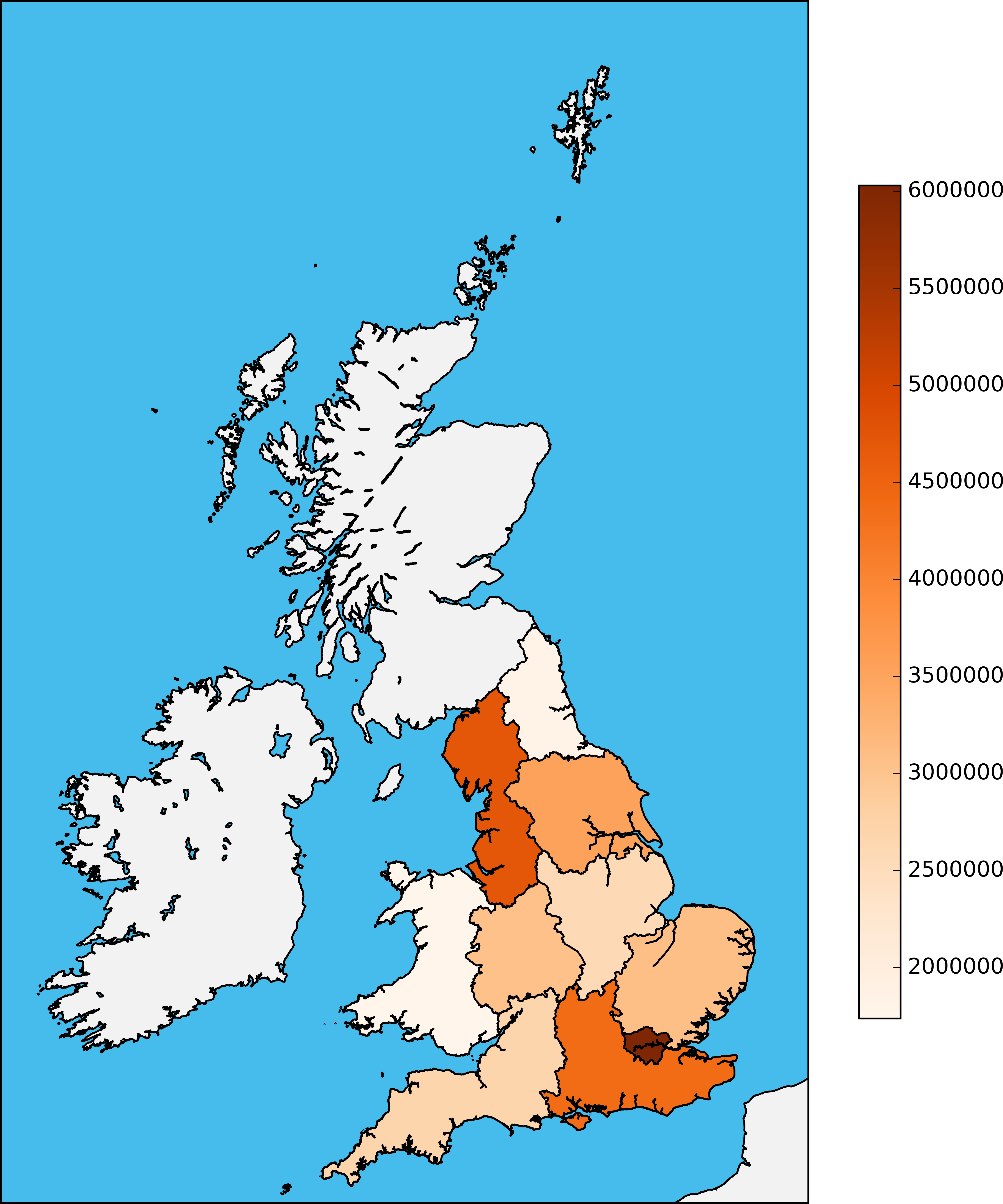
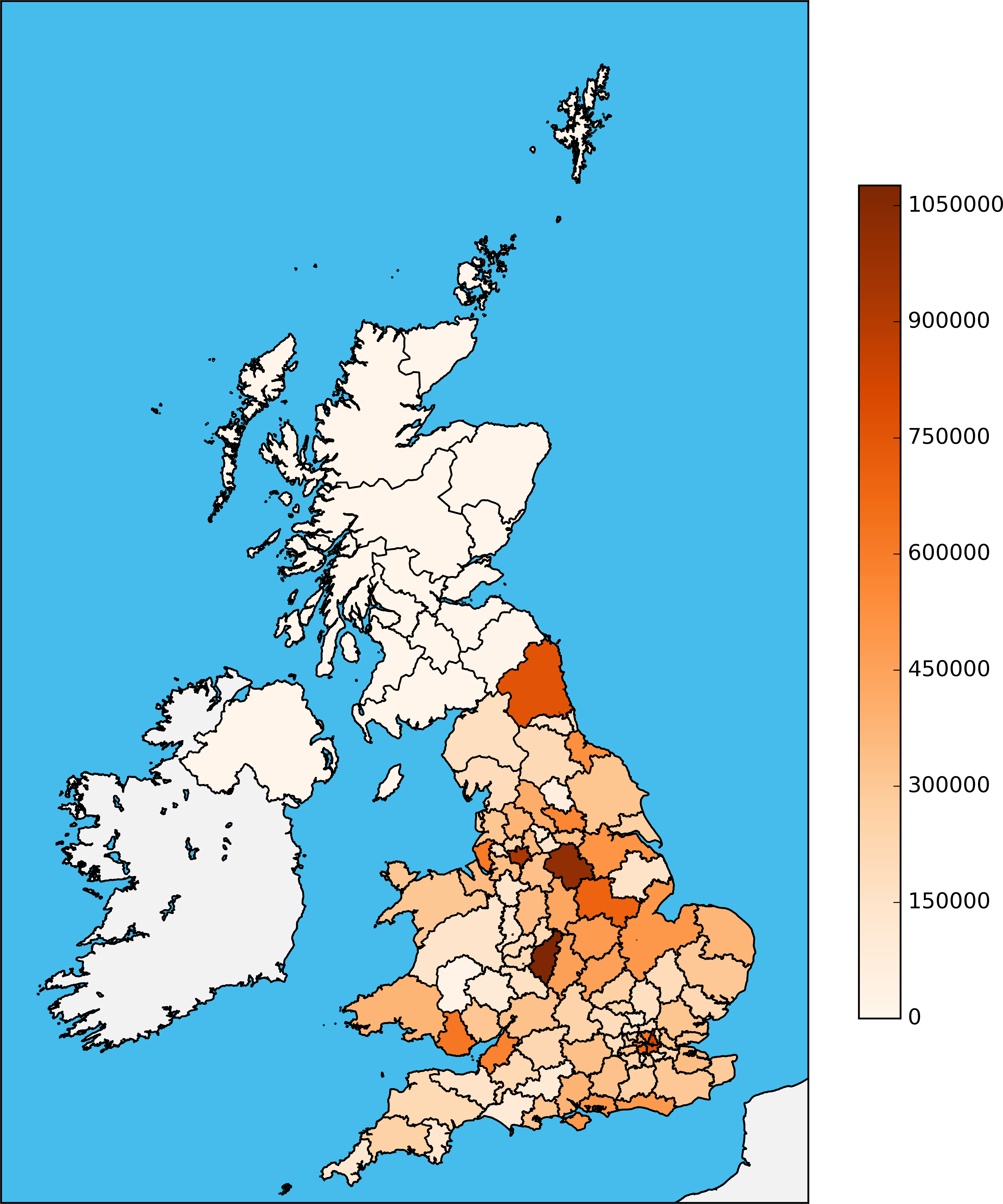
Having those data, we could generate our first map visualizations. The following two images show the absolute number of crimes in the respective areas. The first image is the map of the regions of the UK, while the second is the map of postcode areas.

First Approach for Predicting Crime Outcome Types

In this week we also wanted to execute first prediction experiments with the current data. The main purpose was to get a better understanding of the data, rather than designing a fully reliable predictive model. Given our limited computational resources, we narrowed our experiment to the city of London. The size of the subset is 9.9 MB with 21.662 samples. We also wanted to experiment with only a subset of all features, rather than the 79 Features we currently have. For this approach we chose the following setting:

• Input features:
  • Crime type
  • Number of stop and searches within 500 m reach from the crime with an outcome type "suspect arrested" or "offender given drugs possession warning" or "suspect summonsed to court"
  • Number of Points of Interests (POI) within 500 m reach from the crime
• Target feature:
  • Crime outcome type

For this experiment, we chose a random forest classifier that fits a number of decision tree classifiers on various sub-sample sets and then lets them vote to label a new data point. We chose to conduct this experiment using the Machine Learning library “Scikit Learn” in Python. In this library, decision trees (hence also random forests) expect continuous input, which therefore treats categories as being ordered.

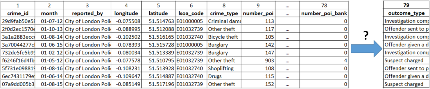
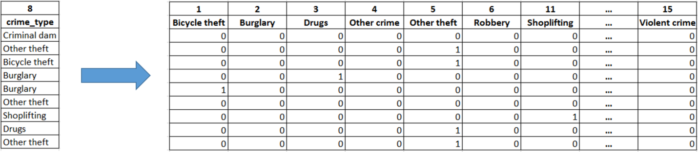
Since we already have two categorical features in our sitting i) crime type as an input feature and ii) crime outcome type as our single target feature, we needed to first preprocess those features before using them in the random forest by encoding them as integers. Afterward, we used the oneHotEncoder and LabelBinarizer provided in the Scikit Learn library for transforming the data. Those encoders transform each categorical feature with x possible values into m binary features, with only one set for each sample (Documentation). As a result of the preprocessing process we had the following:

• The categorical input feature “crime type”, with its 15 possible values, is transformed to 15 binary features using OneHotEncoder
• The categorical target feature “crime outcome type”, with its 8 possible values, is transformed to 8 binary features using LabelBinarizer

Afterward, we concatenated the 15 binary features of the transformed “crime type” feature together with the other input features to use them as an input for training the random forest. The total number of decision trees used in the random forest was 10.

In order to get an estimate of the generalization error on new crime samples, we used cross-validation during the training phase. We calculated the mean of the resulting scores: 59%. We then used our trained random forest to predict the test dataset and got an accuracy of 95.9%. In addition, we calculated the weighted F1-score for the prediction model and achieved: 0.76478.

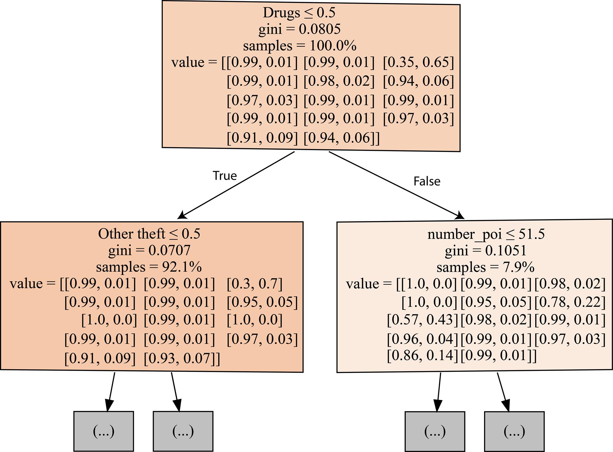
The figure below represents the first three nodes of the first decision tree in the random forest. In each node, the algorithm tries to find the optimal feature, using the gini index, for splitting the data set to reach a better classification. The gini index measures the misclassification (impurity) of the model in a given node. For example, the first node splits the data by considering the crime type “Drugs”. The values in the first node specify the probabilities of the input samples (misclassification prob., correct classification prob.) for each crime type.

Link to Code

Communication with UK Police

Last week we mentioned that we contacted the UK police after discovering that the published geolocation of crimes can vary till 20 km from the original locations due to privacy reasons. The police support center answered promptly stating that they don’t have that figure to hand. However, they offered we can provide them a full list of statistics we are interested in and they will pass our request over to the Home Office for their consideration. They showed their interest in our approach and asked if our work will be published anywhere they would be able to read.

This week we brainstormed the cooperation possibilities with the UK Police and replied asking for their support in the following issues:

1. What is the average corrected distance of all crime to the chosen anonymised points? (https://data.police.uk/about/#anonymisation)
2. The date (day and/or time) of the crimes? If not possible maybe you can share with us only the day time (E.g. Morning, afternoon, evening, night)?
3. The weather on crime’s date and location. Irrespective of the second point, we can provide you with a weather dataset that you can join and send us the weather for a crime?
4. Age range of the defendant(s)/victim(s) of crimes? (We currently have this information only about stop and search incidents)
5. Ethnicity of the defendant(s)/victim(s) of crimes?
6. Any other possible sort of data that you think it might be helpful for us?

We also stated our willingness to sign a confidentiality declaration about the information they provide us if need.

Link to our presentation