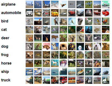
In this example, we will attempt a similar problem as the first example with the MNIST dataset. We will attempt to classify images. Rather than identifying digits in the MNIST dataset, we will use the CIFAR image dataset, which contains thousands of images of ten different objects. Our network will learn to recognize what is in the picture. This is the goal of object recognition and a large part of the computer vision field.

While the basic network in our first example can be used for this task, as the number of samples increases and the number of different classes (objects) to be recognized increases, the fully-connected network layers start failing. It takes longer to train, and the performance starts to degrade.

Convolution layers are another functional element that we can add to neural networks. They work similarly to how image filters work in applications such as Photoshop and GIMP. Let's take a look at how a simple blur filter works.

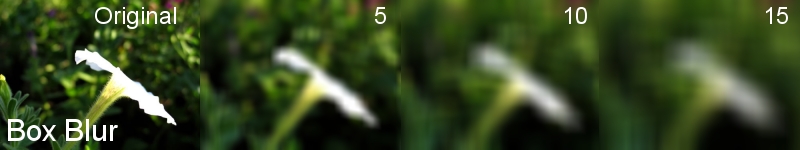
For every pixel in the original image, a filter is passed over it. the new value is the result of averaging all the color values of neighboring pixels in an n×n sized square.

Another blurring technique, called Gaussian blur, works very similarly. A square box is used for every pixel in the original image, and a new pixel color is produced by averaging all the pixels in the box. The difference is that each pixel in the filter is weighted based on how far away it is from the center. In effect, pixels closer to the center affect the output more than those farther away. This leads to a more natural blurring, and avoids artifacts that can be present in the box blur.

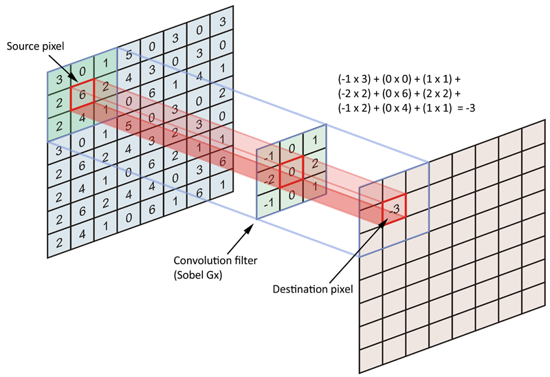
a single convolution layer shown, with an input image, weights, and output pixel

A convolution layer is a similar process. An n×n square is used for every pixel. Every pixel in the filter square has a weight of how much it contributes to the final output. A convolution layers would effectively be a box blur if all of the weights were the same. Additionally, a convolution layer could effectively be a Gaussian blur if the weights in the center were stronger than the weights towards the edge. By passing this filter over every pixel in the original image, we generate a new output image with some convolution filter applied. Many other filters work this way, from blur filters, to edge detection filters, and many more.

Convolution layers leave the weights as trainable parameters. This means that the network will learn what filters would benefit it in its task. For instance, an edge detection filter might help to see outlines of shapes. A blur filter might help to see overall color regions. And the best part is that we, as human beings, don't have to decide exactly what is needed, or how it is used. Like our previous example, we can train the weights in the convolution layer using SGD, iteratively improving the performance of the entire network by slightly tweaking the weight parameters until we are satisfied with its performance. Just as we did in the first example, we can stack multiple convolution layers on top of one another. In fact, there are many different configurations with convolution networks, and each has their merits.

There has also been some work done in exploring what sort of features top-performing convolution networks use to classify images. For instance, these are some images taken at various layers in one of Google's image classifiers:

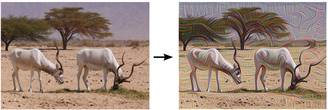
in this image of an antelope, we can see that the network has exaggerated the lines of the original image. Notice how the trees have been transformed into wavy lines.

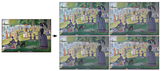
In this image, we can see that the network at different layers has broken the image down in several ways. In one convolution layer, the network has deconstructed the image into sweeping curves (top right), while in another, we see a repetitive texture appearing (bottom left). All of these different views can give the network different information about an image. They all accentuate different features of the original image, which can be better used to classify it, rather than relying on the raw pixel data.

It is important to understand the power of convolution networks do not apply only to images. Other domains, such as audio waveforms, have also seen great benefit from convolution networks. The important characteristic is that there is localized information. In an image, neighboring pixels share a lot of meaningful information. They are related in some way by their proximity to one another. In an audio sample, there may be 44,000 individual samples per second, and neighboring samples also are related to one another by their proximity in time. A convolution can extract meaningful features from this localized data, which aids in the network's tasks.

First off, we need to import TFLearn. For convenience, we will also directly import several modules we will be using a lot

# Import TFLearn and subcomponents
import tflearn
from tflearn.data_utils import shuffle, to_categorical
from tflearn.layers.core import input_data, dropout, fully_connected
from tflearn.layers.conv import conv_2d, max_pool_2d
from tflearn.layers.estimator import regression
from tflearn.data_preprocessing import ImagePreprocessing
from tflearn.data_augmentation import ImageAugmentation

Next, we need to load the data into our program. As before, TFLearn already includes the CIFAR-10 dataset we will be using, se we don't need to download a large file onto the disk.

# Data loading and preprocessing
from tflearn.datasets import cifar10
# Load the data from tflearn package
(X, Y), (X_test, Y_test) = cifar10.load_data()
# Randomize the image order. like shuffling a deck of cards
X, Y = shuffle(X, Y)
# Like the one_hot encoding used for MNIST data
Y = to_categorical(Y, 10)
# Like the one_hot encoding used for MNIST data
Y_test = to_categorical(Y_test, 10)

Due to the relatively limited amount of images we have to work with, it is likely for a network to overfit the training data. What that means is that it learns very specific features about our input, that don't really apply to any other images. For more about overfitting, see here

To combat overfitting, we are going to augment our dataset. In other words, we are going to make many more training images by slightly modifying the original images. The modifications we will do here are randomly flipping them along the Y axis (left-to-right) and slightly rotating them. This will give slightly different images than the original, and we can do this as many times as we need to get a large enough dataset.

As usual, TFLearn has something already set up for us to automatically augment data. We just need to define a new image augmentation scheme, which we will specify later as a parameter to our training function.

# Real-time data augmentation
img_aug = ImageAugmentation()
img_aug.add_random_flip_leftright()
img_aug.add_random_rotation(max_angle=25.)

We also would like to preprocess the images a bit.

# Real-time data preprocessing
img_prep = ImagePreprocessing()
img_prep.add_featurewise_zero_center()
img_prep.add_featurewise_stdnorm()

We first need to introduce a few new functions that we will be using as part of our network.

After a convolution layer, often you will want to reduce the size of the image vector, also known as down-sampling. This reduces the complexity and increases run time performance as you train. The idea being by reducing the size of the data, we can reduce the number of parameters in the latter stages of the network, and reduce our computational overhead. A common down-sampling approach is max pooling. The image is divided into non-overlapping sections, and the largest value in each section is selected as the new value.

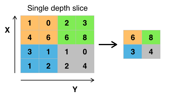
Max pooling an 4x4 image down to a 2x2 image, (2x2 regions being pooled together)

In our network, we made use of two max pooling stages, with a 2x2 sized regions.

As we build our network, we made use of dropout. This is a technique to avoid overfitting. It is a regularization technique. Not all of the neurons in our network are very useful. Dropout is a way for some neurons to be "disabled," letting other neurons do more of the work. A certain percentage of neurons are disabled, depending on their contribution to the final output, which can be calculated to some degree through calculus (which TensorFlow does for us).

# Convolutional network building
input = input_data(shape=[None, 32, 32, 3], # our image data is 32x32 pixels with 3 color channels, RGB
                 data_preprocessing=img_prep,
                 data_augmentation=img_aug)
conv_layer_1 = conv_2d(input, 32, 3, activation='relu') # apply a 3x3 filter on our image, and we will use 32 different filters at this layer (that means the output is a 32x32x32 vector, one 'channel' for each filter)
maxpool_1 = max_pool_2d(conv_layer_1, 2) # maxpool with a 2x2 pooling region size (now 16x16x32)
conv_layer_2 = conv_2d(maxpool_1, 64, 3, activation='relu') # apply a 3x3 filter on our image, with 64 filters (now 16x16x64)
conv_layer_3 = conv_2d(conv_layer_2, 64, 3, activation='relu') # a 3x3 filter on our image, with 64 filters (still 16x16x64)
maxpool_2 = max_pool_2d(conv_layer_3, 2) # maxpool with a 2x2 pooling region size (now 8x8x64)
fully_connected_1 = fully_connected(maxpool_2, 512, activation='relu') # layer of 512 rectified linear units
fully_connected_1 = dropout(fully_connected_1, 0.5) # dropout rate of 50%
output = fully_connected(fully_connected_1, 10, activation='softmax') # final layer, one node for each of the 10 image classes. we use softmax as with the MNIST classifier
optimizer = regression(output, optimizer='adam',  # Adam is an improvement on SGD, however the principle is the same.
                 loss='categorical_crossentropy', # rather than mean squared error, we use a different loss function
                 learning_rate=0.001)

finally, we will train the network for 50 runs through the data.

# Train using classifier. shuffle the data, and use train with a batch size of 96 images at a time.
model = tflearn.DNN(optimizer, tensorboard_verbose=0)
model.fit(X, Y, n_epoch=50, shuffle=True, validation_set=(X_test, Y_test),
      show_metric=True, batch_size=96, run_id='cifar10_cnn')