Object Characteristics - 3dct/open_iA GitHub Wiki
This document describes how to compute a labeled volume and object characteristics, as required by FeatureScout.
FeatureScout requires at least a .csv file describing the characteristics of the analyzed objects; optionally, along with a labelled image. If only the .csv file is available, only the model-based visualizations (cylinder, ellipse) can be used in FeatureScout.
The MObjects feature as well as the labeled objects visualization require a labeled volume. Such a labeled volume needs to fulfill the following requirements:
- It must contain only values between 0 and your number of objects,
- A value of 0 indicates that there is no object at this position,
- Values higher than 0 indicate that at that voxel position, there is an object with that given number; i.e., all voxels belonging to an object need to contain the number representing its object number.
- The mapping from a line in the .csv to an object in the labeled volume happens with the help of this number: The line in the .csv is the ID, which needs to match the number used for labeling the object in the volume.
You can use many image processing tools to create such a labeled volume as described above; here, we describe how you can create a labeled volume with open_iA for a pore dataset; the raw data will be provided soon with the next open_iA release as part of the test datasets.
-
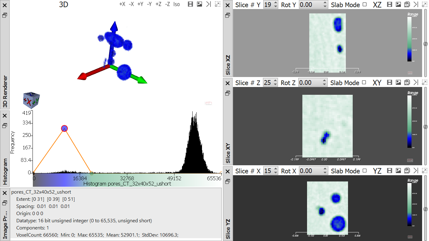
Load the dataset; the example dataset comes with a descriptor file (.mhd). If you have a raw file, you might be asked to enter the dimensions (width, height and depth as well as spacing in x, y and z direction, etc.). See File Formats for more details on the formats supported by open_iA.
-
First, use a filter resulting in a binary mask, indicating where the objects are situated. We can inspect the dataset using the transfer function to find out where to set appropriate thresholds:
-
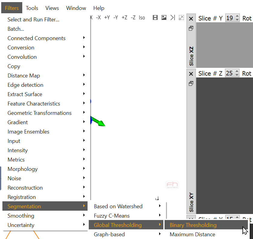
In our case, where the dataset has a good contrast between objects and other materials, we can use the "Binary Thresholding" filter. (Filter -> Segmentation -> Global Thresholding):
-
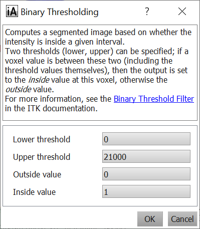
The lower and upper threshold should indicate the range of intensity values inside the pore; these will be assigned the "Inside value", all others the "Outside value":
-
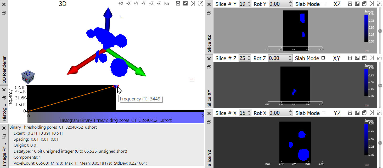
After this step, you get a binary labeled volume (where all voxels where there is an "object" are marked with 1, and all others with 0):
-
In case you have an image with worse contrast, you can play around with many other filters that open_iA provides in the Filter -> Segmentation section.
-
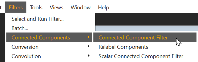
On the binary mask, use a "Connected Component" filter (Filters -> Connected Components) to get individual numbers for each object:
-
There is only one parameter to set, which for our example can be left unchecked:
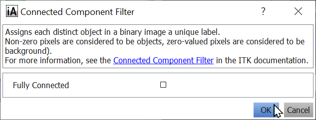
In case you have objects that are 1 pixel wide, consider enabling "fully connected". See the documentation on implementation details linked to in the filter description for more information.
-
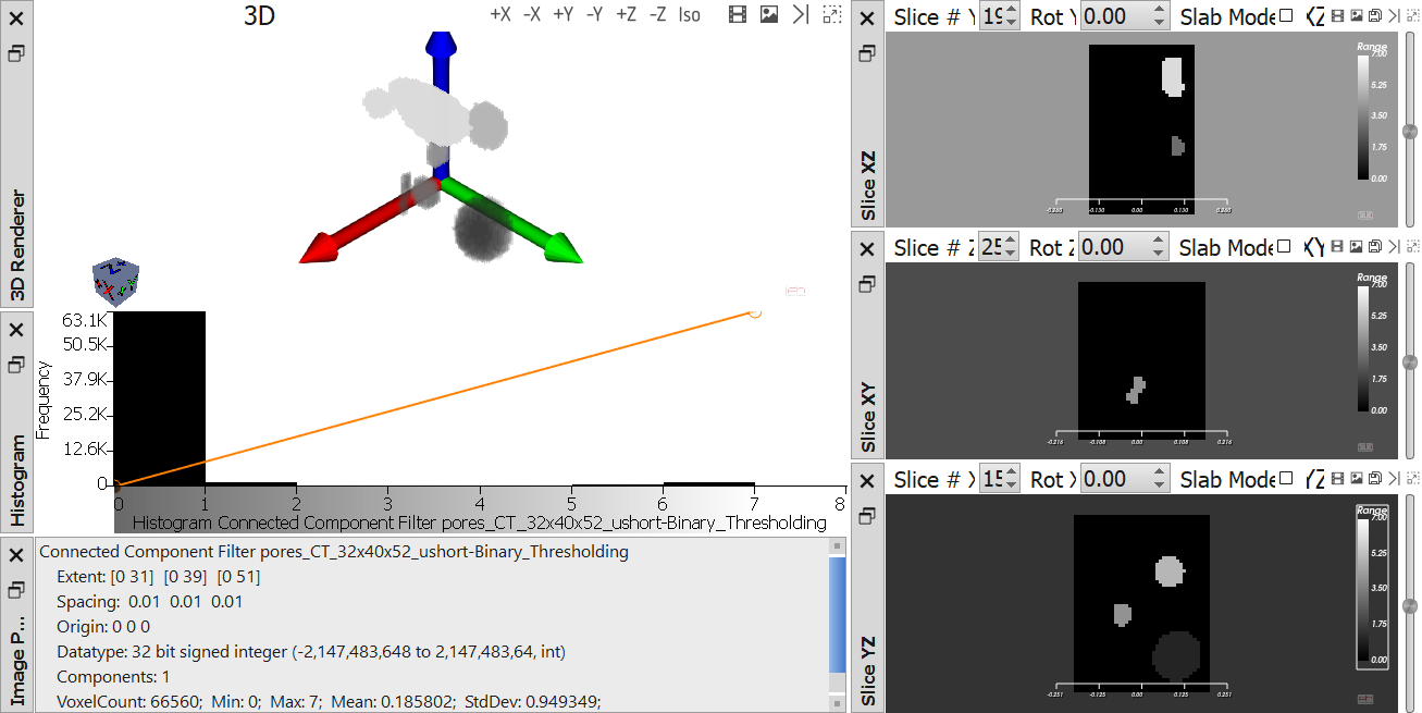
After this step, each object will have its own "number":
-
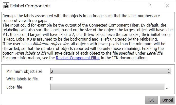
We then typically use a "Relabel Components" filter (Filters -> Connected Components):
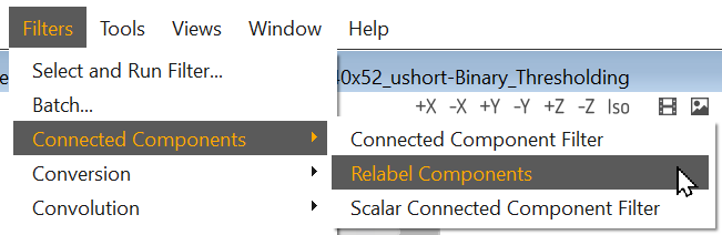
This filter closes any eventual "holes" in the sequential numbering, and (optionally) filters out objects under a certain minimum size:
-
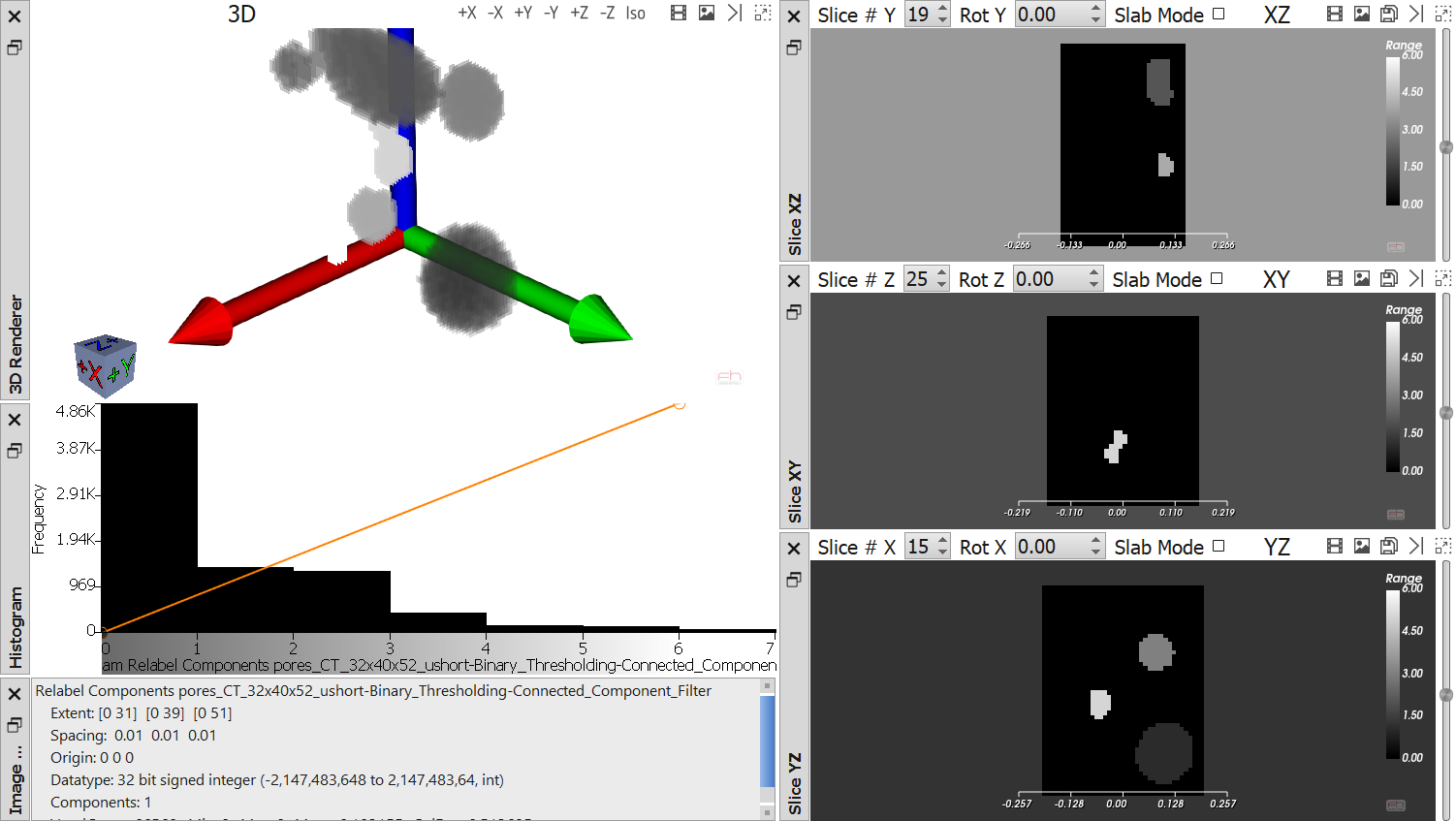
After the filter, the objects (i.e., the according numbers assigned to them) will now be sorted in decreasing order of their size (=number of voxels). You can see that the smallest object with only 1 voxel volume was removed, we now only have 6 objects remaining:
-
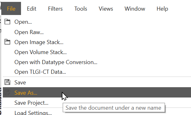
Save the relabeled image (File -> Save As, while the respective sub-window is in focus).
-
You can save it for example in the default-selected "Meta Image" file format.
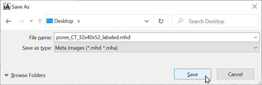
Specify a file with an ".mhd" ending – this .mhd file is a "descriptor" for the also created, linked .raw or .zraw file in the same directory (so that you don't have to specify the raw file parameters anymore). Whether an uncompressed (.raw) or compressed (.zraw) file is created depends on the according setting in the Preferences. Compressed files take less space, but cannot easily be opened by other tools (unless they also support the same compression). Uncompressed .raw files take more space, but are widely compatible across tools for working with volumetric data.
-
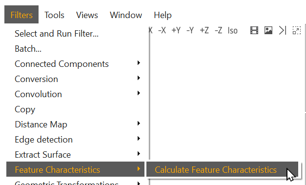
We can now compute characteristics (such as position, length, orientation) of each object, and generate a .csv file with these characteristics per object. Choose Filters -> Feature Characteristics -> Calculate Feature Characteristics.
-
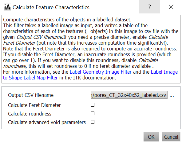
The "basic" options are typically enough (i.e., no need to check any additional checkboxes, as shown below), but make sure to choose a valid file path for the output .csv file, so that you will find again later:
The created files can now loaded in the FeatureScout, to analyze the characteristics distributions in more detail.