GEMSe - 3dct/open_iA GitHub Wiki
Description
GEMSe is a tool for the visualization-Guided Exploration of Multi-channel Segmentation algorithms.
It provides tools to sample the parameter space of a (potentially multi-channel and/or multi-modal) segmentation algorithm; the sampled data can then be analyzed in an exploration interface. This module is the implementation part of a paper published at EuroVis '16, and its extension for arbitrary segmentation algorithms published at the 7th industrial Computed Tomography conference.
Video: https://youtu.be/ggKg3EToGBY
Publications:
- Bernhard Fröhler, Torsten Möller, and Christoph Heinzl, “Visualization-Guided Exploration of multi-channel segmentation algorithms”, Computer Graphics Forum, Vol. 35, No. 3, pp. 191–200, June 2016, doi: 10.1111/cgf.12895.
- Bernhard Fröhler, Christoph Heinzl, Johann Kastner, Torsten Möller, "Parameter-Space Exploration for Computed Tomography Image Analysis Algorithms", 7th Conference on Industrial Computed Tomography (iCT2017), Leuven, Belgium, 2017, url: ndt.net/?id=20856.
Usage Scenario
Suppose you have a multi-channel image, as for example from
- A Talbot-Lau Grating Interferometer Computed Tomography device (with Attenuation, Phase Contrast and Dark Field channels)
- An MRI image (with T1, T1c, T2, Flair channels)
- A Hyperspectral Image (with > 100 channels from different wavelength spectrum bands)
You now want to find the most suitable segmentation, taking the information from all channels into consideration. The pipeline of GEMSe to achieve this consists of two steps:
- Preprocessing: Sampling the parameter space
- Analysis: Exploring the result and parameter space
Note: The following descriptions apply for open_iA >= 2016.09. For version 2016.06, please refer to an older version of this guide
Preprocessing
Step 1: Load the Modalities
Before sampling can be started, all information channels need to be loaded in open_iA. Each data channel is taken from an individual volume (3D image):
-
Open the first 3D image via File -> Open.
-
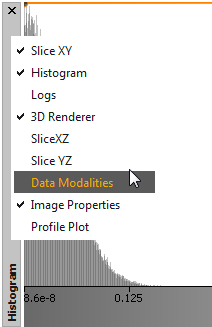
Go to "Data Modalities" widget. If it is not visible, open it through right-clicking on the title bar of one of the dock widgets:
images/dockwidget-titlebar-contextmenu-datamodalities.png
See the Layout section in the user guide in case this doesn't work.
-
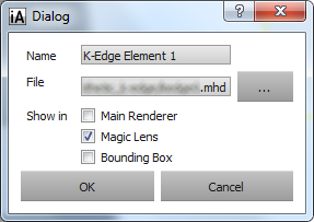
Click the "+" button to add an additional modalities. In the opening dialog:
-
Select the file to add (either by entering the full filename or by selecting it with the dialog appearing when pressing "...").
Note: The file needs to show the same object and needs to be pre-registered to the first dataset.
-
Give the modality a name.
-
You can select any of the "Main Renderer", "Magic Lens" and "Bounding Box" checkboxes, these determine where the data is shown.
-
The dialog could look like this:
-
Repeat step 3 for all modalities you want to use in the pipeline.
Step 2: Sampling
-
Select Tools -> Image Ensembles -> GEMSe (open_iA < 2018.4: Tools -> GEMSe or Tools -> Segmentation Ensembles -> GEMSe); the "GEMSe Control" widget should get visible.
-
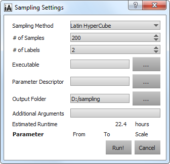
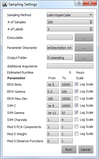
Click the "Start..." button in the "Sampling" row of the "GEMSE Control" widget to open the Sampling Configuration dialog:
-
Specify the "Number of Samples": this is the amount of runs of the full pipeline that are going to be performed, so depending on the size of the dataset, you might want to choose a number appropriate for the time you allow the sampling to take.
-
Specify the "Number of Labels". Currently, GEMSe does not perform a check whether the label images actually contain this amount of labels; the color-coding used for the label images will be limited to this number, so make sure to input a number equal or bigger than the actual label number.
-
Specify an "Executable". The program entered here will be called for each generated parameter set. See GEMSe Algorithms for details, e.g. on the order of arguments.
-
Specify a "Parameter Descriptor". This is a file that contains a description of all parameters that the given executable accepts and that should be sampled over. For more details, see the Parameter Descriptor File Format. As soon as the path to a valid parameter descriptor file is entered, the sampling dialog will update to show sampling ranges for all described parameters:
images/GEMSe-sampling-settings-dialog-parameter-descriptor-loaded.png
-
Specify an output directory; GEMSe will pass a subfolder of the given one (/sample) to the executable.
-
Specify arbitrary "Additional Arguments" that the selected executable might need.
-
If you want you can adapt the parameter ranges. Their default are the ranges specified in the Parameter Descriptor file (see d.)
-
The default sampling method is "Latin Hypercubes", which tries to best cover the parameter space. Other sampling methods ("Random" and "Cartesian grid") are also available.
-
Start Sampling by pressing "Run".
-
Depending on the data size and the used command, the sampling can take quite some time. Be prepared to let it run over night or over the weekend. GEMSe will provide a useful estimate on the remaining time after the run of the executable with the first parameter set has finished.
-
In addition to the segmentation results, GEMSe will also calculate derived measures in the form of the count of connected components as "object count" out of resulting label images.
After a sampling run is finished, all results, are stored in the given output directory. In addition, a sampling overview file (*.smp) is created, which describes the parameters and ranges used during sampling. The sampling run can be loaded again from this overview file in later sessions.
Step 2.5: Combine multiple sampling runs
You can combine multiple sampling runs in the analysis, to compare different algorithm pipeline outcomes. To add another sampling run:
- Either load it via the "Load..." button in the "Sampling" row of the "GEMSE Control" widget
- Or create another one, by repeating steps 2.-5. of the previous section.
Step 3: Clustering
- Make sure all sampling runs you want to include in your analysis are loaded
- Press "Cluster" button in the "GEMSe Control" widget.
- You will be asked to specify a output directory for the clustering results
The clustering will be stored as clustering file (*.clt) in the specified output directory. Furthermore, a GEMSe project file (.sea) will be created, which references all samplings used for clustering using relative paths. You can use this project file to load previously calculated samplings at a later point in time.
Analysis
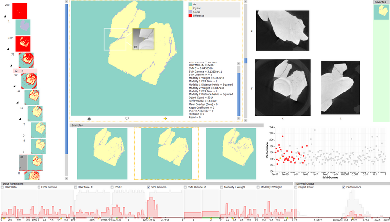
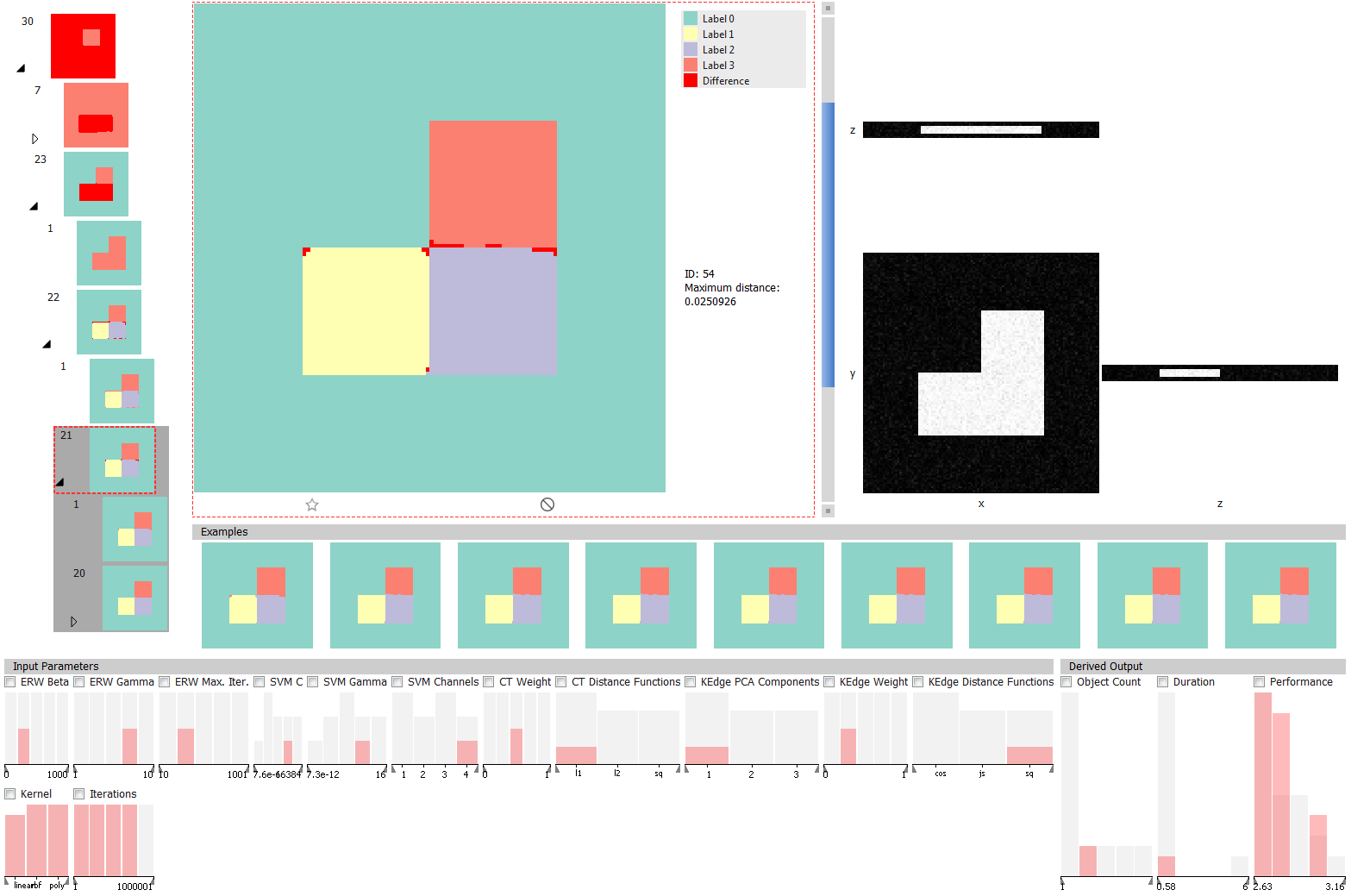
When clustering is finished or a previously calculated results are loaded (via "Tools" menu, "GEMSe" -> "Load Pre-Calculated Results"), the analysis interface is shown. With a simple synthetic dataset loaded it looks like this:
images/GEMSe-analysis-synthetic.png
For a detailed description of the views and their interaction, please refer to the paper linked to above.
See also the GEMSe module code.
Back to Tools.