Tutorial 3 Full PUMA Main Rotor - zanoni-mbdyn/blendyn GitHub Wiki

PUMA full main rotor model

In this tutorial will be animating a full aeroelastic model of the main rotor of an Aérospatiale SA 330 Puma helicopter. The full model of the PUMA is available through the MBDyn website here (scroll down to the "Applications" section), while the model that we will be using is distributed with the Blendyn add-on, in the tests/puma_rotor directory of the repository.

Simulate the model and locate the results file

The main input file for the model is called puma-4blade-elastic. As was the case in the helicopter blade analysis tutorial, the NetCDF output is enabled by activating the related option in the control data section of the input file

begin: control data;
	...
	output results: netcdf;
 end: control data;

Again, this is not strictly necessary, but let's say highly recommended: it speeds up considerably the loading of the MBDyn output, and it enables plotting of variables directly in Blender.

As shown in the other tutorials, after you have simulated the model, you want to import first the .nc or .mov file, and then the .log file, in order to give the add-on all the necessary information about the MBDyn model structure.

Import nodes and elements

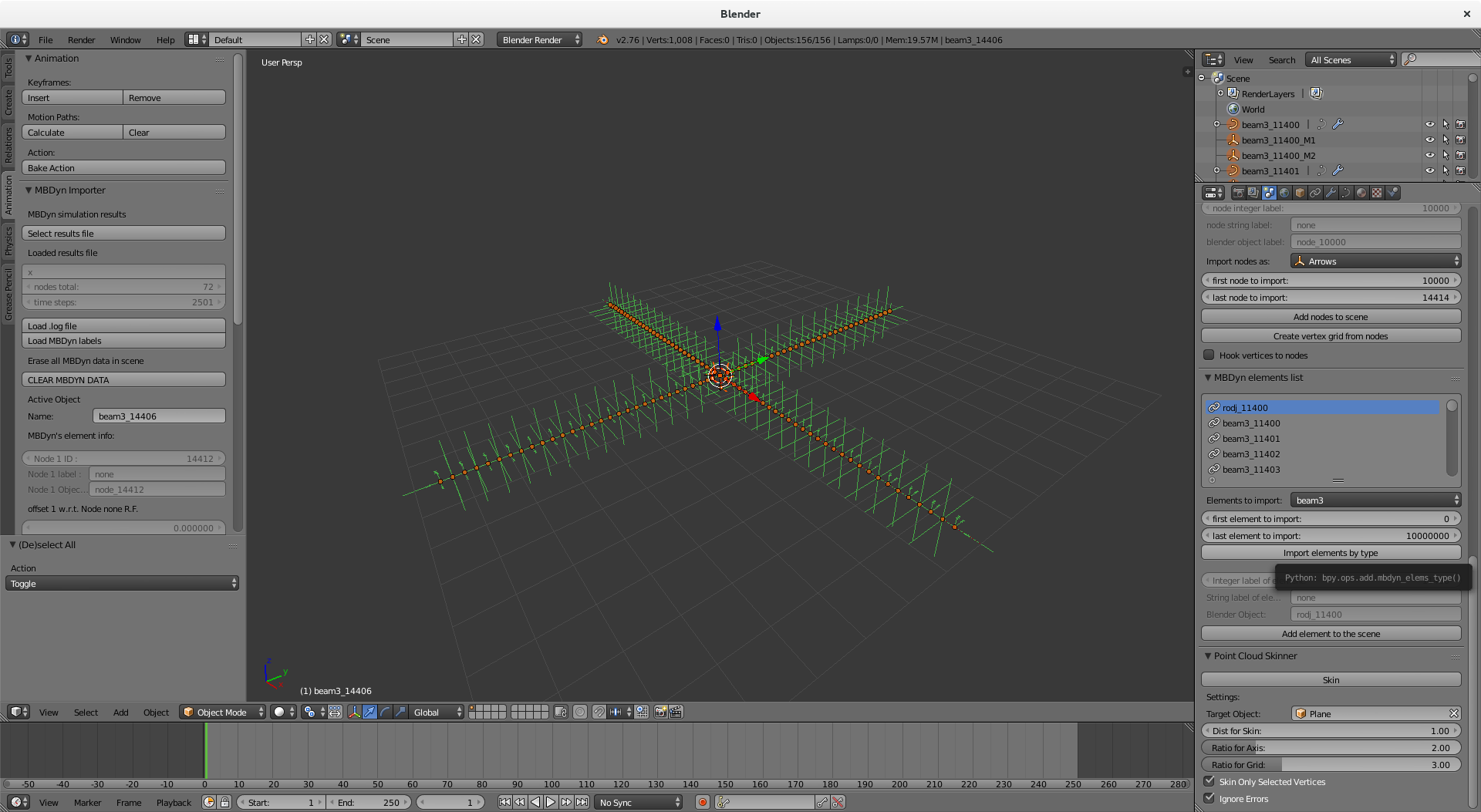
Switch to the Scene Property panel and scroll down until you see the MBDyn nodes and elements lists. Click on the Add nodes to scene button to import all the nodes as empty axes. You should get something similar to what is shown in the following picture

By selecting Individual Origins as the Pivot centers for scaling and rotation, pressing S and dragging the mouse, the dimensions of the empties axes can be reduced.

OK, so now we have the first hint that we're dealing with an helicopter rotor.

In the MBDyn model, the blades are modeled with beam3 elements, to take into account their deformation. We can import all the beam3 elements at once by going to the Scene Properties Panel, scrolling down to the MBDyn element list, select beam3 in the Elements to import drop-down menu, inserting a random big number in the last element to import field and click on Import elements by type button. The result is shown in the following picture

The beam elements have been imported as NURBS curves, as explained in helicopter blade analysis tutorial and in the wiki page about the import of beams.

The plain axes empties are auxiliary objects used in the animation of beam3 elements that can be hidden by manually selecting them in the Scene Outline and pressing H or by clicking on the small eye found next to their names. You can also use some very simple python commands to do so from the python console:

for obj in D.objects:
	if 'M1' in obj.name:
		obj.hide = True

and repeating that for the second set of auxiliary objects:

for obj in D.objects:
	if 'M2' in obj.name:
		obj.hide = True

The same procedure can be used to import the four rod elements representing the pitch links. This time, as explained in the wiki page on the rod joints import, the deformable elements are represented as straight 3D lines in space.

The model's base structure is already evident: if you'd so like, you can animate the scene by pressing on Animate scene in the Tool Panel. The output of the simulation consists in 2501 steps, that can take quite a bit of time to load. Setting the frequency to something around 10 (i.e. to animate one frame every 10 simulated steps) will result in a manageable number of frames. If you want to output the final result in a video file, keep in mind that you should instead select a frequency according to the framerate of the movie. Standard framerates are 24, 25 or 29.97 fps, so (considering that the final time of the simulation is 4.5 seconds), you should set the frequency to 2501/(4.5*24) = 23, 2501/(4.5*25) = 22 or 2501/(4.5*29.97) = 18, respectively.

'Dressing up' the model

Ok so now it is time to dress up the model, to make it look a bit more like an helicopter rotor :)

Blade airfoil profile

First of all, let's grab a suitable profile for the blades. Head to Airfoiltools and click on NACA 5 digit airfoils on the left sidebar. Scroll down and download the Selig format dat file for the NACA 23012 12% arifoil. Save the file in the blender model folder (actually, you can save it wherever you like, but we like to keep things tidy, here).

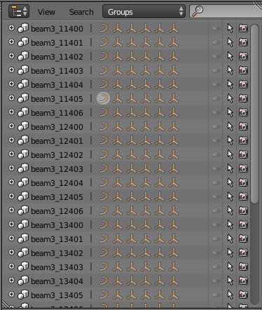
Then, you want to select all the beam curves. You can head to the Group Outliner, as shown in the following picture, and click on all the curve icons next to the name of the beam groups, holding the SHIFT key:

or you could use some Python trickery again. First, deselect all by pressing A (possibly, more than once). Then, head to the Python console and type

for obj in D.objects:
    if 'beam' in obj.name and 'M' not in obj.name:
        obj.select = True

Now press the Load profile (Selig) button in the Data Properties panel:

and locate the NACA 23012 Selig-formatted file you saved before. The profile is automatically assigned as a bevel shape for all the selected beam curves. You should have something similar to what is shown in the next picture

The profile curve is placed on the first empty layer: in this case, layer 2. We want to scale it down to the correct dimensions and move the origin of blender reference frame of the curve object to the correct position. If you have taken your time to take a peek in the MBDyn model files, you might have noticed that the parameters for the aerodynamics of the rotor blades are written in the blade.set file, in particular at line 44:

44 set: const real blade_chord     = 0.537;        # m

we want to scale the profile to have that length. Since profiles loaded in Selig format have unit cord length, we want to scale the shape uniformly by a factor 0.537. Just select the curve and enter 0.537 in the Scale fields (all of them) in the Transform Panel.

Then, we want to move the origin of the axes attached to the section to a quarter of the chord length: in the Location fields of the Transform Panel place -0.25*0.537 in the x direction, to move the profile to the left of that quantity. Now make sure that the cursor is in the origin (for example with Shift + S -> Cursor to Center), press Shift + Alt + Ctrl + C and select Origin to 3D Cursor. You should now have something similar to what is shown in the screenshot below

Now, moving back to layer 1, the blades should now look a lot more realistic. To add a little bit more of realism, let's add a taper profile to the beams closer to the root of the blade.

Switch to layer 3 and create a NURBS curve with the parameters shown in the next screenshot

You can define your own shape at will. What worked for me are the following (X, Y) coordinates for the four points (named progressively from left to right):

1 (0.0, 0.35)
2 (0.35, 0.35)
3 (0.6, 1.0)
4 (1.0, 1.0)

You may want to rename the object you just created to something more telling, like BladeTaper or something similar.

Select, one at a time, the blade root beams (the objects named beam3_ 11400, beam3_12400, beam3_13400, beam3_14400) and select the NURBS curve you just created as a taper object. You should have something similar to the screenshot below

Now select the tip beams' objects (objects names beam3_11406, beam3_12406, beam3_13406, beam3_14406) and select the Fill Caps option, to close the blade tips with a solid face. The checkbox is also located in the Geometry Panel.

Pitch links sections

For the pitch links, we want a very simple bevel curve: a circle of diameter 2 cm. Select layer 4, add a circle and give it Size 0.02 in all directions. Now select it as the bevel objects for the pitch links' rods (objects rodj_11400, rodj_12400, rodj_13400, rodj_14400) and select as a bevel object for each the circle you have just created.

Rotor Head

In the tests/puma_rotor/cad directory of the repository, a full CAD 3D model of the PUMA rotor head is provided. Well, actually the model provided is that of a PUMA-like rotor head, since both geometry and dimensions, aside from the ones that really matter for the purposed of matching with the MBDyn model, are arbitrarily guessed... Anyway, it will serve our purposes fine!

You can also find the CAD assembly on Onshape at this link: you are free to copy, share, export and build upon the model under the terms of the CC Share Alike licence.

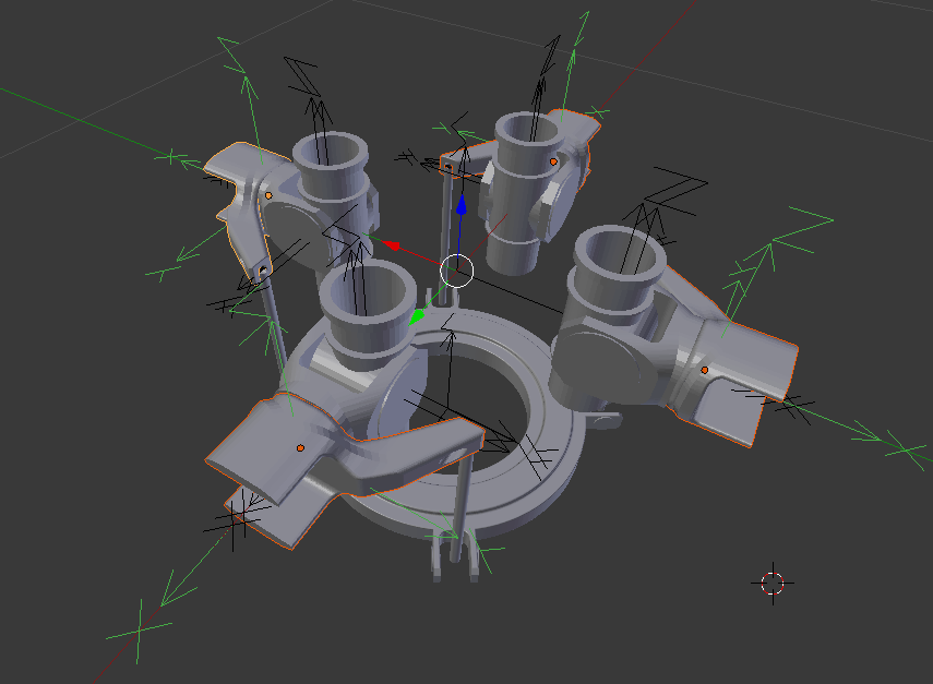
The tags in the figure reflect the name of the .stl files the CAD assembly has been split into, each containing the geometry of a component represented in the MBDyn model by a node.

Swashplate rotating disc

Let's start by loading in Blender the swashplate.stl file. Go to File->Import...->Stl (.stl) and locate the file. After the import, Blender will automatically select the file. The default units in the .stl files are millimiters, while the MBDyn models uses meters, so we have to scale the mesh by a factor 0.001. Press S and type 0.001, then press Return to do so.

Another thing that we want to do is to place the local axes of the swashplate mesh in the correct position. By going into Edit Mode (hitting TAB), you can notice that the origin of the mesh geometry is already in the correct location, while by returning into Object mode (again hitting TAB) you'll notice that the origin of the Object is not. Simply hit Shift + Alt + Ctrl + C and select Origin to Geometry to fix the local axes origin. Hit R, then X and type -90 and press return to fix also the axes orientation, placing the Z axis upward. Hit Ctrl + A and then select Rotation to apply the rotation, re-defining the reference orientation of the Object.

The node representing the rotating swashplate is node 10300: you can work it out by looking at the set statements in files puma.set, hub.nod and puma-4blade-elastic, or just watching at the central part of the rotor, moving between frames of the animated Blender model. We want to place the swashplate Object in the same location and with the same orientation of the Empty representing its node: select it by clicking on the object named node_10300 in the Scene Outline. Hit Shift + S and select Cursor to Selected to move the cursor in the origin of the node's Empty Axes. Then select the swashplate Object, hit again Shift + S and select Selection to Cursor.

Next, rotate the swashplate Object about its Z-axis (by pressing R and then Z) to align it: place the pitch links approximately in the center of their joint sections, for now.

Lag hinges

Let's now focus on the lag hinge: import the lag_hinge.stl file and scale the mesh as before. Hit Shit + Alt + Ctrl + C and select Origin to Geometry: also in this case, this is all you need to do to place the local axes in the correct position.

Now, to align the local axes with respect to the MBDyn node, rotate the mesh by 90° about the X-axis and by 180° about the Z-axis to get the mesh in the orientation shown in the screenshot:

Apply the rotation by pressing Ctrl + A and selecting Rotation.

Select the first lag hinge node Empty Object, which is node_11100, press Shift + S, select Cursor to Selection. Then select the lag hinge mesh, press again Shift + S and this time select Selection to Cursor. This way, you will have moved the lag hinge mesh in the correct position.

Now double check that you have only the lag hinge Object selected and hit Shift + D to duplicate it. Select the second lag hinge node Empty Object node_12100, hit Shift + S, select Cursor to Selection... You got it: just repeat the process to position also the second lag hinge Object. To align it, apply a rotation about the Z-axis of 90°, to match the orientation of the node_12100 Object.

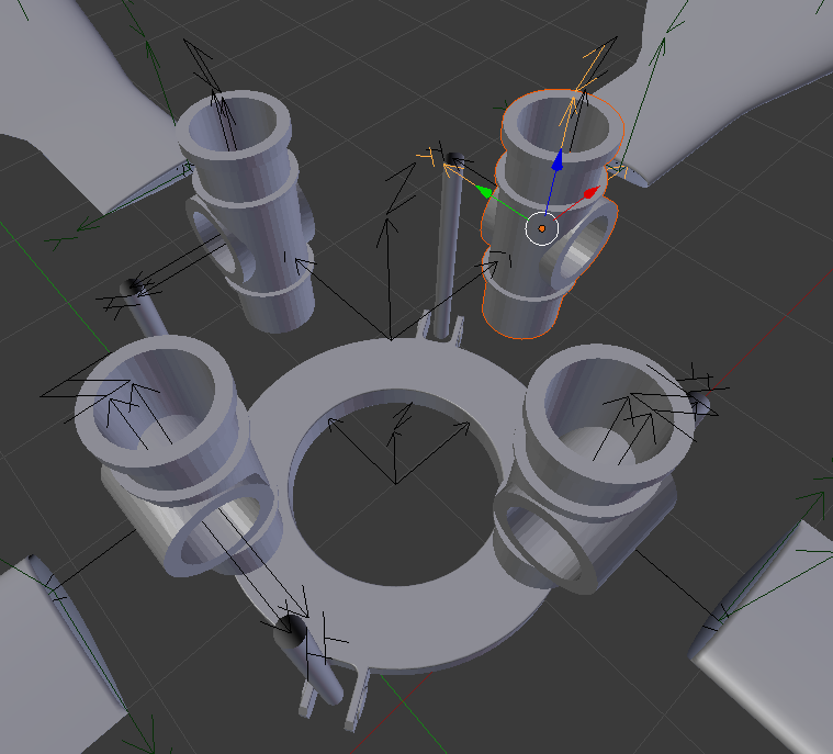
Repeat the process for the other two lag hinges, and you'll what is shown in the following screenshot

All is left to do is to assign the correct parenting: select the lag hinge object first, the node Object second holding Shift (this way, the node Object will be the active Object) and then press Ctrl + P and select Object to set the parenting. In the outline, the parenting will be reflected by the mesh object being moved under the node Object in the tree.

So for example for the first lag hinge, after you have selected the mesh Object, hold Shift and select the node_11200 object. Move the cursor to the 3D View and hit Ctrl + P and select Object. Repeat the process with the others lag hinges.

Flap hinges

Import the flap_hinge.stl file, scale it and tab into Edit Mode: we want to place the local reference frame in the middle of the fork, on the axis passing though the centers of the cilindrical sections that protrude at each side. To do so, let's first place the reference frame where the central vertex of the outside faces of the cylinders is (look at the next image):

Then do the usual procedure to align it with the first flap hinge node Empty Object node_11200: select the node_11200 Object, hit Shift + S and click on Cursor to Selected, then select the flap hinge object, hit again Shift + S and select Selection to Cursor. You'll get to this configuration:

Click on the Y-axis of the flap hinge Object (the green arrow) and drag it to place it in the correct position. If you did not move the Cursor in the process, directly press Shift + Alt + Ctrl + C and select Origin to 3D Cursor. If you happened to move the Cursor, first place it back in the node_11200 origin by selecting the Object and, as usual, pressing Shift + S and selecting Cursor to Selection, then proceed to move the origin of the flap hinge Object.

Duplicate the flap hinge mesh and repeat the process, aligning all the meshes to the nodes' Empties. Assign the parenting as you've done for the lag hinges.

Pitch hinge

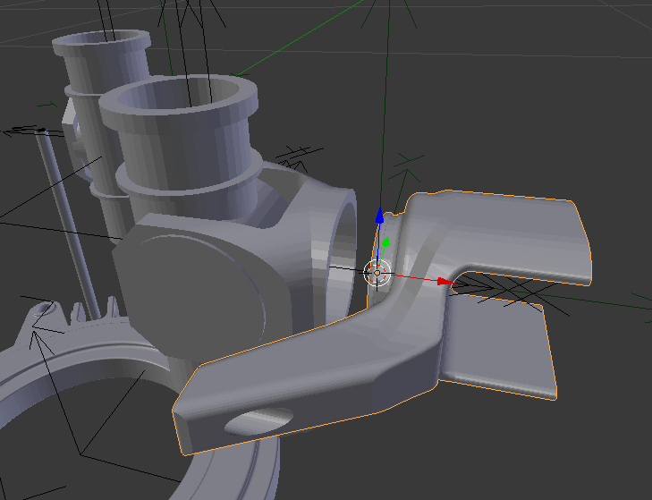
As you did before, load the pitch_hinge.stl file, scale it down by a factor 0.001, hit Shift + Alt + Ctrl + C and select Origin to Geometry, place the mesh in the same location of the node_11400 Object and rotate it to match the node orientation. You'll get to this configuration:

You just have to move the mesh by dragging the red arrow to align the sections of the flap hinge and the flap hinge. Also make sure that the pitch link joint is correcly aligned with the pitch link rod! As done for the other hinges, duplicate the object, place them in the correct positions and assign the parenting to the node_11400, node_12400, node_13400 and node_14400 Objects.

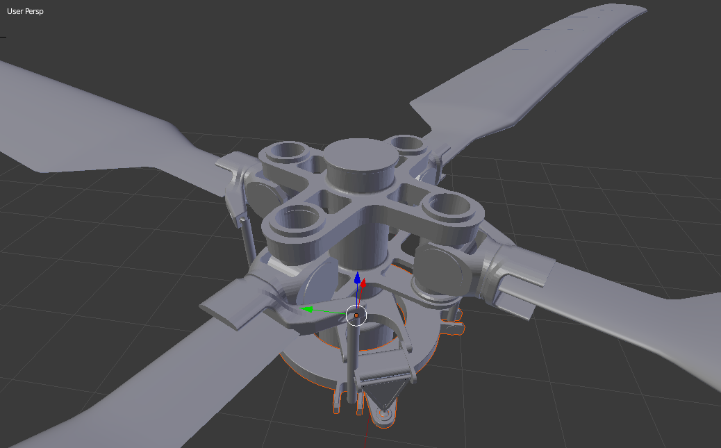
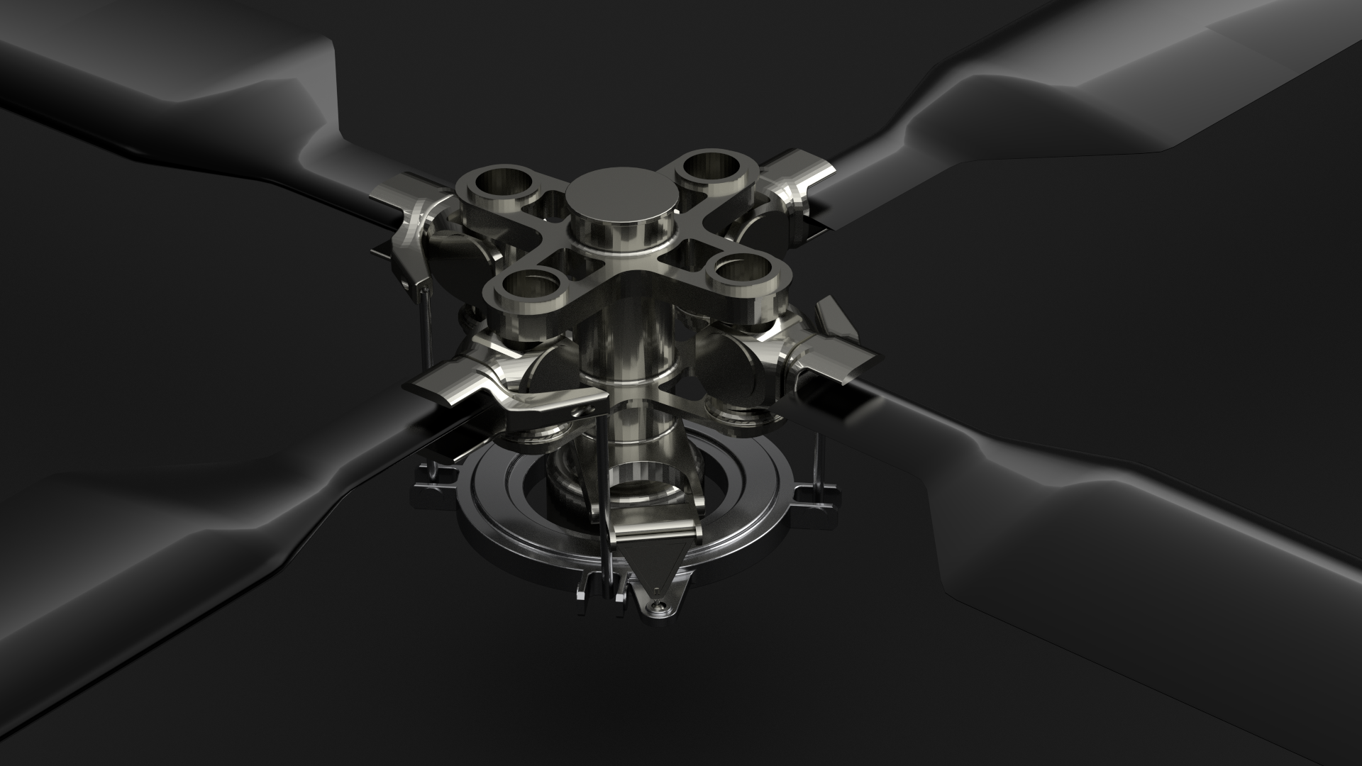
We have completed the positioning and parenting of the rotor hinges: you should have something similar to this:

Rotor hub

The last piece that we have to place and parent is the hub mesh, that you can find in the hub.stl file. The node that represents this rigid body is node_10300. The procedure is the same as the swashplate and the hinges meshes: import the file, scale it, move the local axes to the Geometry axes, rotate it to have the Z axis pointing upward, select the node_10100 Object, move the cursor to its origin, then move the hub Object to the cursor. You should have to then move the mesh along the Z axis and rotate it about the same axis to mate it with the hinges and swashplate meshes: you'll find the correct position by matching the lag hinges with their seatings and the compass ball joints and their seatings. Don't forget to parent the swashplate Object to the node_10300 Empty Axes Object and the hub Object to the node_10100 Empty Axes Object, and you should get to something similar to this:

... And that's it! The model is ready to be animated! Best of things, it won't require any other adjustment as you go through different simulations: as long as you don't rename the nodes in the MBDyn input files, you can just load a new result file and animate the Blender scene again!

Renders

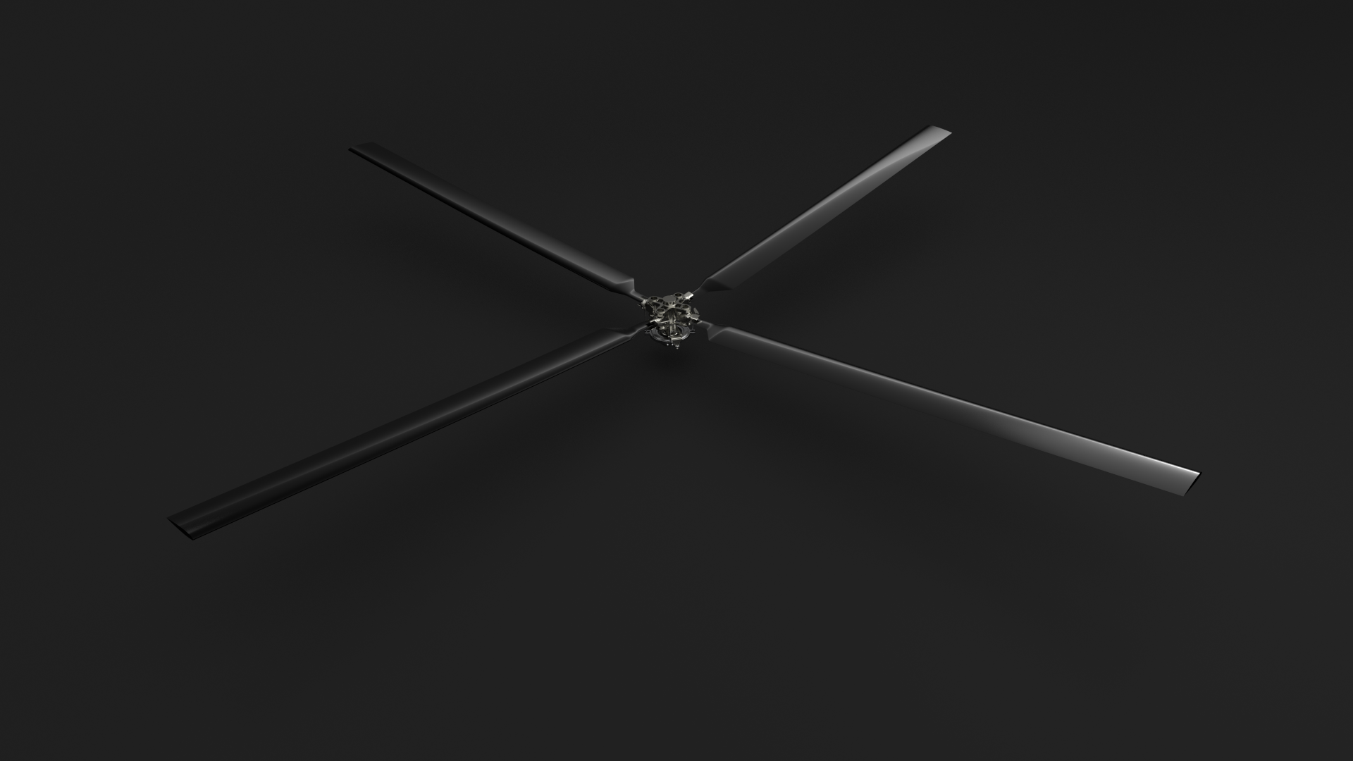
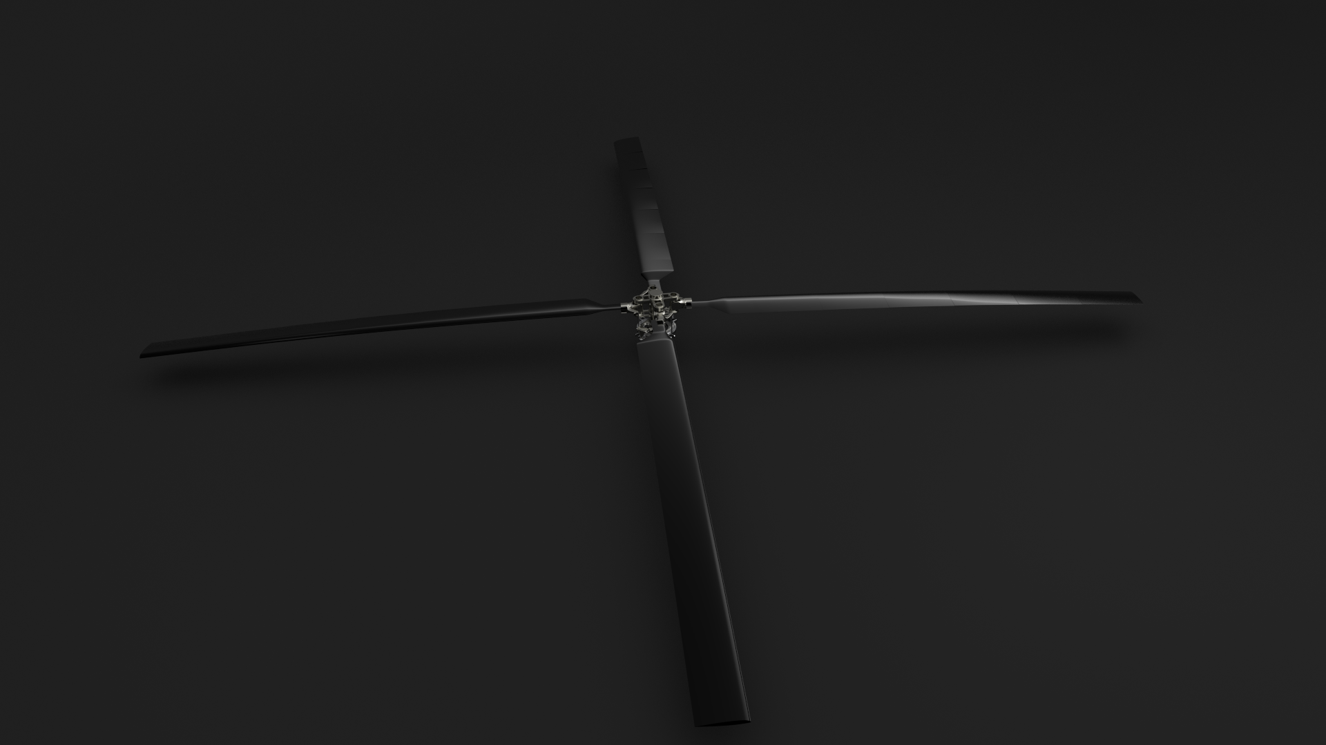
Just some images (and soon animations): I simply added some materials to the bladed and the rotor head assembly, some lights and a camera, and rendered the result. Send a request if you're interested and I'll share the final .blend file.

Happy Simulations :)