DNN Architecture - yszheda/wiki GitHub Wiki
Systolic Array
Systolic Architectures
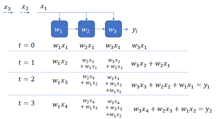
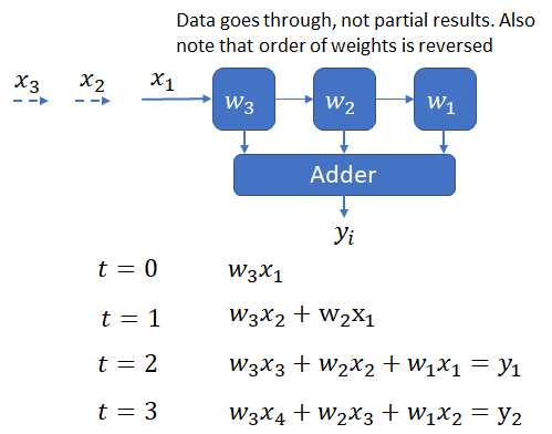
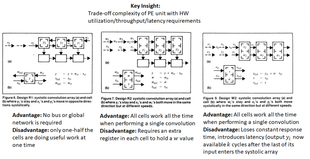
weight stationary: A downside of both these designs is that either each element of the input must be broadcast to all PEs (in the first design) or the partial outputs must be collected and sent to the accumulator. Doing so requires the use of a bus, which must scale as the size of the correlation window increases.
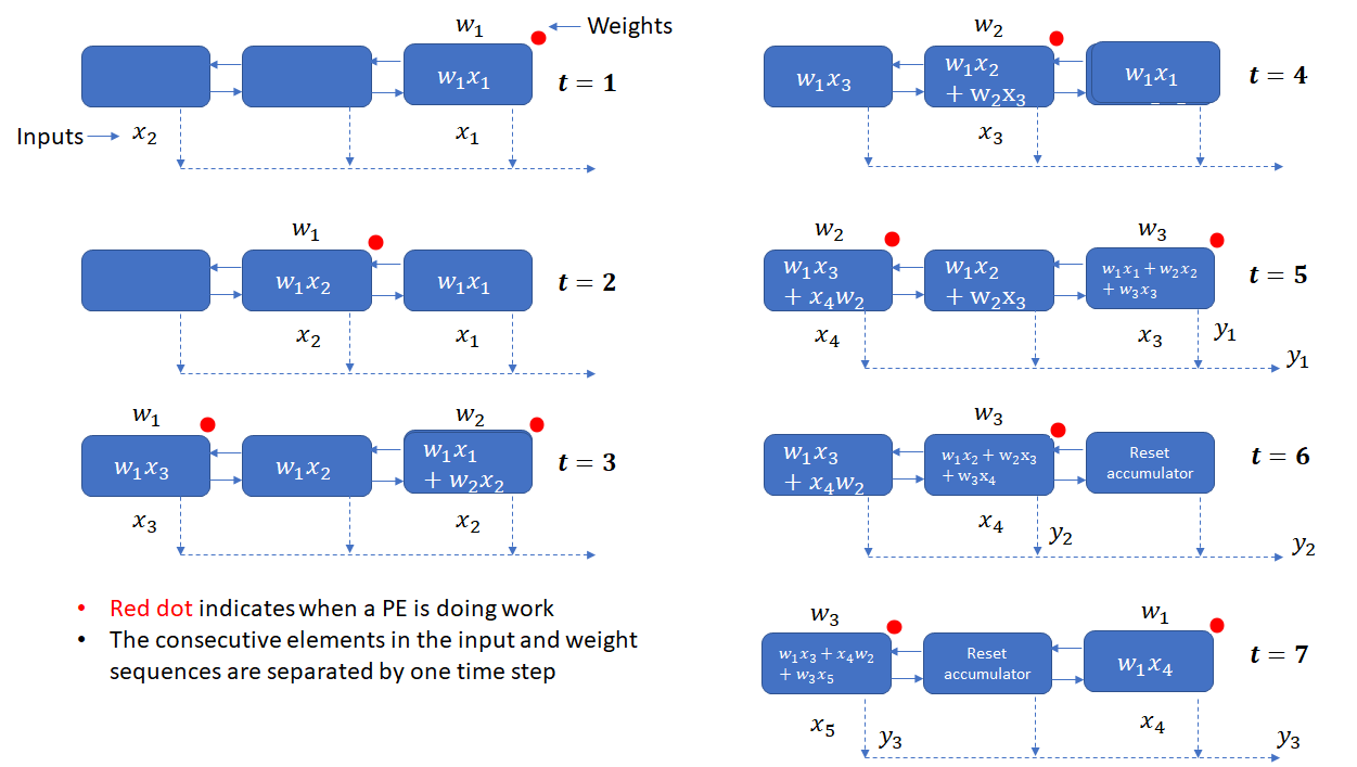
output stationary: This design doesn’t require a bus or any other global network for collecting output from the PEs. A systolic output path, indicated by the broken arrows is sufficient. While this design solves the problem of the global bus, it suffers from the drawback that each PE is performing useful work only one half of the time (as indicated by the red dots). Extra logic is also necessary to reset the accumulator in a PE once it completes calculation of a y_i.
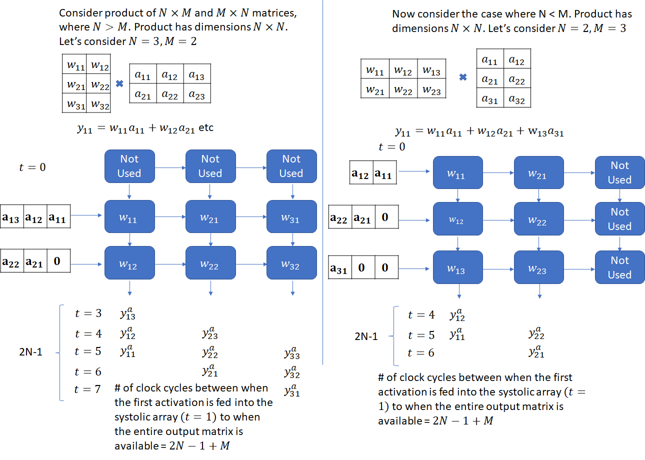
Matrix Multiplication on a Weight Stationary 2D Systolic Array (MXU on a Google TPU)
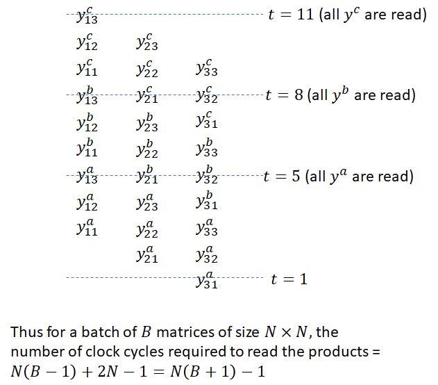
It takes 2N-1 cycles to read all elements of the product of two N x N matrices.
Advantages and Disadvantages of a TPU
Disadvantages
- Latency Depends on Matrix Dimensions
- Poor MXU Utilization and Wasted Memory BW for Non-Standard Matrix Dimensions
- Implementing Convolutions as Matrix-Multiplications may not be Optimal
- No Direct Support for Sparsity
Pipelining of Weight Reads
The basic idea is to load the weights for the next network layer while processing the computations for the current layer. The TPU implements a 4 tile weight FIFO to transfer the weights from the off-chip DRAM to the on-chip unified buffer. The matrix unit is double-buffered so it can hold the weights for the next layer while processing the current layer.
Simulator
- https://scalesim-project.github.io/tutorials-2021-isca.html
- https://github.com/scalesim-project/scale-sim-v2
Notes on "SCALE-Sim: Systolic CNN Accelerator Simulator"
III. B. Modelling Dataflow

Output Stationary (OS)
The data is fed from left and top edges of the array, where the left edges stream in input pixels while the top edge streams in pixels from the filter or weight matrices. In a given column PEs in each row are responsible for generating adjacent output pixels in a single channel. Each column however generates pixels corresponding to different output channels.
Weight Stationary (WS)
The mapping takes place in two steps. First each column is assigned to a given filter. For a given column, the elements of the assigned filter matrix are fed in from the top edge, till all the PEs in the given column has one element each. After the filter elements are placed, the pixels of input feature map are then fed in from the left edge. During this phase, the partial sums for a given output pixel is generated every cycle. For a given output pixel, the corresponding partial sums are distributed over a column. These partial sums are then reduced over the given column in next n cycles, where n is the number of partial sums generated for a given pixel. The weight pixels are kept in the array until all the computations which require these values as operands are not over. Once the computations corresponding to the mapped weight are done, the mapping is repeated with new set of weights.
- The number of SRAM banks needed to support this implementation is lower than output stationary implementation for a given array.
- However, partial sums corresponding multiple output pixels are now required to be kept in the array, until they are reduced, which leads to increase in implementation cost.
Input Stationary (IS)
Similar to WS, this mapping also takes place in two stages. However, in this case, each column is assigned to a convolution window. The Convolution window is defined as the set of all the pixels in the IFMAP which are required to generate a single OFMAP pixel. As in the case of WS, for a given column the pixels corresponding to a given convolution window are streamed in from the top edge. Once the input pixels are fed in, the elements of the weight matrices are streamed in from the left edge. Again similar to WS, reduction is performed over a given column, and the convolutions windows are kept around until all the computations requiring these elements are done, before remapping the array with elements belonging to new convolution windows.
- This dataflow also enjoys the benefits of lower SRAM bank requirements, as compared to OS.
- However the cost and runtime compared to WS varies by workload.