Data Transformation Techniques

Part of MMM’s appeal is that it is grounded in key marketing principles, such as adstock and saturation, where these principles are further reflected in Robyn:

Adstock

This technique is very useful for a better and more accurate representation of the real carryover effect of marketing campaigns. Moreover, it helps us understand the decay effects and how this can be used in campaign planning. Adstock reflects the theory that the effects of advertising can lag and decay following an initial exposure. In other words, not all effects of advertising are felt immediately - memory builds and people sometimes delay action until following weeks, where this awareness diminishes over time.

Saturation

The theory of saturation entails that each additional unit of advertising exposure increases the response, but at a declining rate. This is a key marketing principle that is reflected in MMM and Robyn as a variable transformation.

You can find more technical details on both of these here, including the underlying equations. It is important that you understand the meaning of each hyperparameter correctly before fine-tuning and adjusting it - if unsure, you can simply use our recommended settings as described below.

Adstock Techniques

There are two adstock techniques you may choose from in Robyn, each with its pros and cons. In order to find the approach that best fits your model objectives and business purposes, we recommend testing various transformations.

Geometric

The biggest advantage of the Geometric transformation is its simplicity. It only requires one parameter called ‘theta’ that can be quite intuitive. For example, an ad-stock of theta = 0.75 means that 75% of the impressions in period 1 were carried over to period 2. This can make it much easier to communicate results to non-technical stakeholders. In addition, Geometric is much faster to run than Weibull, which has two parameters to optimize.

However, Geometric can be considered as too simple and often not suitable for digital media transformations, as shown in this study. When it comes to setting hyperparameters for a Geometric transformation technique, theta is the only parameter that can be adjusted, which reflects the fixed decay rate. For example, assuming TV spend on day 1 is 100€ and theta = 0.7, then day 2 has 100x0.7=70€ worth of effect carried-over from day 1, day 3 has 70x0.7=49€ from day 2 etc. A general rule-of-thumb for common media channels are:

• TV = c(0.3, 0.8)
• OOH/Print/Radio = c(0.1, 0.4)
• Digital = c(0, 0.3)

Weibull

While the traditional exponential adstock is very popular, it was recently reported by Ekimetrics & Annalect that the Weibull survival function / Weibull distribution can better fit modern media activity such as Facebook. The Weibull survival function / Weibull distribution provides significantly more flexibility in the shape and scale of the distribution. However, Weibull can take more time to run than Geometric, as it optimizes two parameters (i.e. shape and scale) and it can often be difficult to explain to non-technical stakeholders without charting.

When it comes to setting hyperparameters for the Weibull transformation technique, this will depend on which type of Weibull transformation:

• Weibull CDF adstock: The Cumulative Distribution Function of Weibull has two parameters - shape & scale. It also has a flexible decay rate, whereas Geometric adstock assumes a fixed decay rate.

  • The shape parameter controls the shape of the decay curve, where the recommended bound is c(0.0001, 2). Note that the larger the shape, the more S-shape and the smaller the shape, the more L-shape.
  • The scale parameter controls the inflexion point of the decay curve. We recommend a very conservative bound of c(0, 0.1), because scale can significantly increase the adstock’s half-life.

• Weibull PDF adstock: The Probability Density Function of the Weibull technique also has two parameters in shape & scale, and also has a flexible decay rate as Weibull CDF. The difference to Weibull CDF is that Weibull PDF offers lagged effects.

  • For the shape parameter:
    • When shape > 2, the curve peaks after x = 0 and has NULL slope at x = 0, enabling lagged effect and sharper increase and decrease of adstock, while the scale parameter indicates the limit of the relative position of the peak at x axis;
    • When 1 < shape < 2, the curve peaks after x = 0 and has infinite positive slope at x = 0, enabling lagged effect and slower increase and decrease of adstock, while scale has the same effect as above;
    • When shape = 1, the curve peaks at x = 0 and reduces to exponential decay, while scale controls the inflexion point;
    • When 0 < shape < 1, the curve peaks at x = 0 and has increasing decay, while scale controls the inflexion point.

While all possible shapes are relevant, we recommend c(0.0001, 10) as bounds for shape. When only strong lagged effects are of interest, we recommend c(2.0001, 10) as bound for shape.

When it comes to scale, we recommend a conservative bound of c(0, 0.1) for scale.

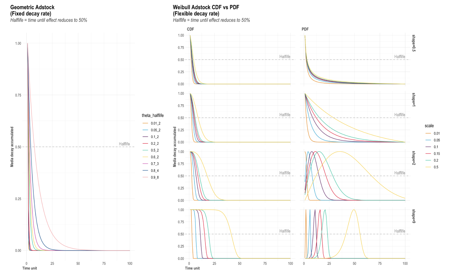
Due to the great flexibility of Weibull PDF and more freedom in hyperparameter spaces for Nevergrad to explore, it also requires a large number of iterations for modeling.

If the description above is too complicated, you can access the adstock helper plot in Robyn which visualizes how the three adstock options Geometric, Weibull CDF & Weibull PDF are transforming the data as the parameter changes. See below for example charts:

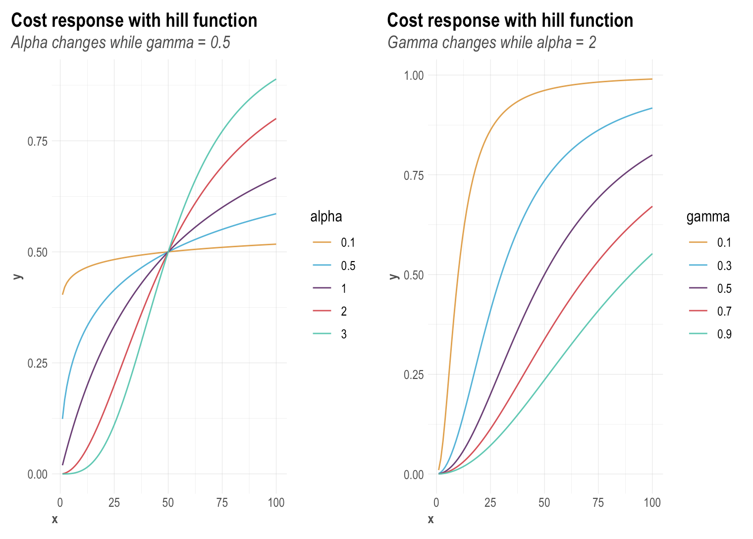
Saturation

Robyn utilizes the Hill function to reflect the saturation of each media channel. A Hill function is a two-parametric function in Robyn with alpha and gamma:

• Alpha controls the shape of the curve between exponential and s-shape. We recommend a bound of c(0.5, 3) - note that the larger the alpha, the more S-shape and the smaller the alpha, the more C-shape.
• Gamma controls the inflexion point. We recommend a bound of c(0.3, 1) - note that the larger the gamma, the later the inflection point in the response curve.

You can also access the helper plot to see how the Hill function transforms as the parameter changes - see below for some example saturation charts: