A step by step guide to use spp - xinwang2hms/SPP GitHub Wiki

Here we demonstrate how to use spp to read in ChIP-seq data, calculate cross-correlation profile, compute, preview and save various sorts of profiles. The data we use for this demonstration come from ENCODE project for profiling H3K4me3 and H3K27me3 in mouse (link?). The raw sequencing data have been aligned to mouse genome using Bowtie, and the results are available for download (H3K4me3, H3K27me3, Input).

Global settings

First of all, we load in package spp. If parallel computing is wanted, multicore should be loaded and a variable spp.cores should be set by function options to indicate how many cores to use. If the user wants to save profiles in tdf format, please indicate where igvtools is installed. density.max.points can be set to control the maximal resolution of plots of tag densities and enrichment profiles.

> library(spp)

> library(multicore)

> options(spp.cores=4)

> options(igvtools="/home/xinwang/Software/igv/IGVTools/igvtools")

> options(density.max.points=10000)

Reading in ChIP-seq data

In spp, each sample of a ChIP-seq experiment is represented by an object of class AlignedTags. The class AlignedTags should not be directly used as it is a root class, from which more specialized classes such as BAMTags and BowtieTags inherit. Here, for example, we initialize a BowtieTags object and read aligned tags:

> encH3K4 <- BowtieTags(genome_build="mm9")

> encH3K4$read(file="H3K4me3.btm.bz2")

Brief message will be displayed when you type in the object created:

> encH3K4

BowtieTags object:

30787977 fragments across 21 chromosome(s)

read from file 'H3K4me3.btm.bz2'

Similarly, we can create an object for H3K27me3 and Input sample. The code is omitted here, but let us name these two objects encH3K27 and Input, respectively.

Calculating cross-correlation profile

Next, we calculate strand cross-correlation profile to determine binding peak separation distance and estimate window size that should be used for binding detection:

> encH3K4$compute.cross.cor(srange=c(-100,500), bin=10)

If the global variable spp.cores is set in the first place, parallel computing will be performed here.

The following method can be used to visualize cross-correlation profile:

> encH3K4$view.cross.cor()

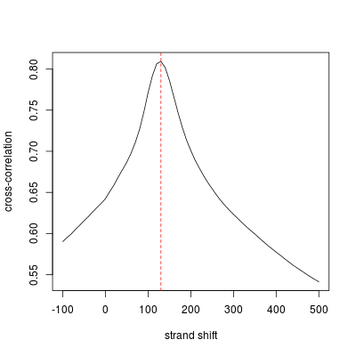
As we see, the peak separation distance is around 130, at which the peak height is much greater than the counterpart at the read length, which is also called 'phantom peaks'. We are now in the process of adding a QC step to quantify the quality of ChIP-seq data by comparing the 'real' peak and phantom peaks.

Now, typing in the object will display in addition information about binding characteristics:

> encH3K4

BowtieTags object:

30787977 fragments across 21 chromosome(s)

read from file 'H3K4me3.btm.bz2'

Binding characteristics:

cross correlation peak: Position=130, Height=0.809

optimized window half-size: 280

Similarly, we should perform the same analysis for encH3K27 and Input.

Quality control

Multiple QC are supported in spp. The method phantomPeak can be used to search for phantom peaks. NSC (Normalized strand cross-correlation coefficient) and RSC (Relative strand cross-correlation coefficient) as well as a quality flag are calculated for quantitative assessment of data quality.

> qc.phantom.peak <- encH3K4$phantomPeak()

NSC=1.49, RSC=1.71, Quality flag: 2

> qc.NRF <- encH3K4$NRF()

NRF=0.62, NRF (no strand)=0.55, NRF (adjusted)=0.8

Previewing tag density profiles

A basic method view is provided to preview smoothed tag density in a specified genomic region. An important feature of view is that no pre-computation of genome-wide density profile is needed before you view a genomic region of interest. However, do pay attention to the parameter step, which controls the sampling density. A very high step will result in a very sparse density profile, whereas a very low step may overuse memory.

> encH3K4$smoothed_density$set.param(bandwidth=1000, step=100)

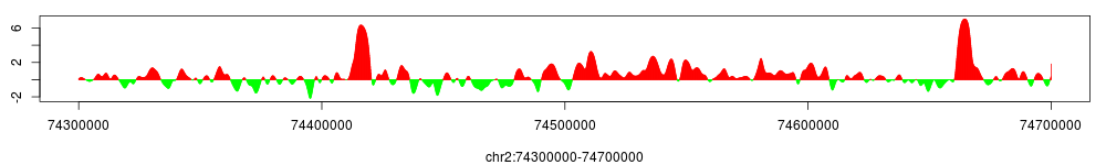
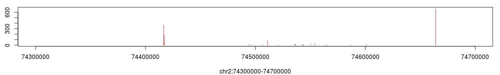
> encH3K4$smoothed_density$view(chr="chr2", start=74300000, end=74700000)

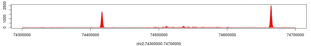
The figure above shows tag density at the HOXD gene cluster. To compare, using the same method we can get the tag density profiles for encH3K4 and Input.

A tag density profile can be saved either in 'wig' or 'tdf' format, which can be imported to igv genome browser:

> encH3K4$smoothed_density$write.wig(file="enc.H3K4me3.smoothedTagDensity.wig", feature="H3K4me3 smoothed tag density", name="ENCODE H3K4me3", zip=TRUE)

> encH3K4$smoothed_density$write.tdf(file="enc.H3K4me3.smoothedTagDensity.tdf", feature="H3K4me3 smoothed tag density", name="ENCODE H3K4me3", save_wig=FALSE)

Profiling smoothed and conservative enrichment

A typic configuration in ChIP-seq data analysis consists of one Input sample and one ChIP sample. Now that we have finished the analysis on single ChIP-seq samples, we next discuss how to use spp to profile enrichment, binding positions as well as broad regions of enrichment.

To start, an object of IPconf should be created by the following code:

> conf <- IPconf(ChIP=encH3K4, Input=Input)

> conf

Input:

24096305 fragments across 21 chromosome(s)

ChIP:

30787977 fragments across 21 chromosome(s)

Binding characteristics:

cross correlation peak: Position=130, Height=0.809

optimized window half-size: 280

As we see, a brief message describing the configuration is displayed when typing in the object. Similar to smoothed tag density profiles as introduced above, to visualize smoothed enrichment profile within a specified genomic region, we can use method view, which performs real time computing:

> conf$smoothed_enrichment$set.param(bandwidth=1000, step=100)

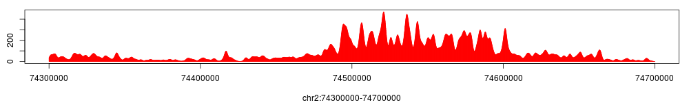
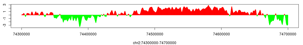
> conf$smoothed_enrichment$view(chr="chr2", start=74300000, end=74700000)

Note that parameter step controls the density of sampling: the larger step is the lower the resolution of the density plot will be. Global variable density.max.points can be set to limit the maximal number of sampling points in the plot, just to avoid heavy computing and using too much memory.

We can preview the conservative enrichment profile using a very similar approach, the only difference being the parameters:

> conf$conserv_enrichment$set.param(fws=3000, bwsl=c(1, 5, 25, 50)*3000, step=100, alpha=0.01, bg_weight= conf$smoothed_enrichment$get.param("bg_weight"))

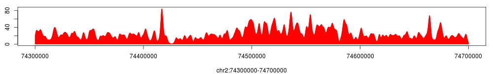
> conf$conserv_enrichment$view(chr="chr2", start=74300000, end=74700000)

Since bg_weight has already been calculated previously when we compute the smoothed enrichment profile, in the code above we just use get.param to retrieve it and set the parameter for conserv_enrichment.

Using the same method, we can preview smoothed and conservative enrichment profile of H3K27me3 at the HOXD cluster:

The method to save smoothed and conservative enrichment profiles in wig or tdf format is the same as smoothed tag density profiles, e.g.:

> conf$smoothed_enrichment$write.wig(file="enc.H3K4me3.smoothedEnrich.wig",

feature="H3K4me3 smoothed enrichment", name="ENCODE H3K4me3", zip=TRUE)

> conf$smoothed_enrichment$write.tdf(file="enc.H3K4me3.smoothedEnrich.tdf",

feature="H3K4me3 smoothed enrichment", name="ENCODE H3K4me3", save_wig=FALSE)

Profiling binding positions

Point binding position profiling in spp is realized in a slightly different way due to the difficulty of real time computing. Instead, the user should expect heavier computation before the profile can be previewed. However, once the profile is computed, it is cached in the object and can be reused unless the user wants to change parameters and re-compute the profile, which can be detected internally by spp (well, hopefully).

> conf$binding_position$set.param(fdr=0.01, method="tag.wtd", add_broad_peak_reg=TRUE)

> conf$binding_position$identify()

Note that identify can be skipped, since it will be internally invoked by other methods such as get.bp and view.bp if binding position profile is not yet in the cache.

The following methods can be used to get binding positions and narrow peak profile as a table:

> bp <- conf$binding_position$get.bp(sort_by="chr")

> narrowpeak <- conf$binding_position$get.narrowpeak(sort_by="chr")

Now that the binding position profile is already in the cache, we should be able to preview:

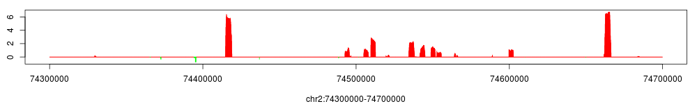
> conf$binding_position$view.bp(chr="chr2", start=74300000, end=74700000)

Methods are also provided to save identified binding positions and the narrow peak profile:

> conf$binding_position$write.bp(file="enc.H3K4me3.bp.txt")

> conf$binding_position$write.narrowpeak(file="enc.H3K4me3.narrowpeak.txt")

Profiling broad region enrichment

As shown in previous plots of enrichment profiles, H3K27me3 is supposed to have a broad binding pattern instead of point binding. In spp, a class broadRegion is designed to handle this task. Since the class is also dependent on ChIPSeqProfile, using this class is quite straightforward as the other classes:

> conf$broad_region$set.param(window_size=1e4, z_thr=3,

bg_weight=conf$smoothed_enrichment$get.param("bg_weight"))

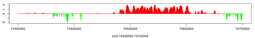
> conf$broad_region$view(chr="chr2", start=74300000, end=74700000)

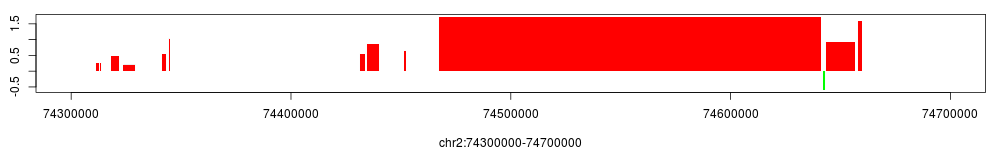
Indeed, as shown in the figure above, we observe a very broad region encompassing the whole HOXD gene cluster.

Broad regions can be saved in the broadPeak format:

> conf$broad_region$write.broadpeak(file="enc.H3K27me3.broadPeak")