Regularization in Machine Learning - vvsnikhil/ML-Blogs GitHub Wiki
One of the major aspects of training your machine learning model is avoiding over fitting. The model will have a low accuracy if it is over fitting. This happens because your model is trying too hard to capture the noise in your training data set. By noise we mean the data points that don’t really represent the true properties of your data, but random chance. Learning such data points, makes your model more flexible, at the risk of overfitting.
Causes of overfitting and how regularization improves it
“Regularization is any modification we make to a learning algorithm that is intended to reduce its generalization error but not its training error.”
Let's take a look at the simple curve fitting problem to understand regularization and over-fitting. Given a set of points (x1,y1),(x2,y2)...(xN,yN). Our goal is to find a model, which is a function y=f(x) that fits the given data. To do this, we can use the method least-square error.
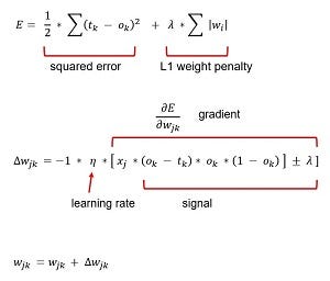
For simplicity, suppose f(x) is just a first order linear function, f(x)=Wx+b. Our job is to figure out what W and b are. We set up an error function that looks like:

To figure out what W and b are, we need to minimize the error function above. However, in minimizing the error function, we get into a problem called over-fitting, when the model we found fits very well with the training data but fails miserably if we apply new data (i.e, get another set of data points).
To do this, we introduce a new terms into the error function, which implies that the coefficient W are also derived from a random process. The error function now looks like:

The added term is call the regularized term that penalizes the large weights.
To illustrate, suppose f(x) can be any order. To generate testing data, we first have a function y=g(x). Next, from points belonging to y=g(x), we added some noise and make those points our training data. Our goal is to derive a function y=f(x) from those noisy points, that is as close to the original function y=g(x) as possible. The plot below shows over-fitting, where the derived function (the blue line) fits well with the training data but does not resemble the original function.

After using regularization, the derived function looks much closer to the original function, as shown below:

Here are the common ways to regularize models.
1. L1 Regularization aka Lasso Regularization–This adds a penalty term with a parameter λ in the error function that we need to reduce. W is nothing but the weight matrix here.Here, λ is a hyper parameter whose value is decided by us. If λ is high it adds high penalty to error term making the learned hyper plain almost linear, if λ is close to 0 it has almost no effect on the error term causing no regularization. L1 regularization is often seen as a feature selection technique too as it zero out the respective weights of features undesired. L1 is also computationally inefficient on non-sparse cases.
2. L2 Regularization aka Ridge Regularization— L2 regularization may not seem quite different from L1, but they have almost non similar impact. Here weights ‘w’ are squared individually and then added. L1’s feature selection property is lost here but it provides better efficiency on non-sparse cases,parameter λ works same as L1. Coefficient of parameters can approach to zero but never become zero.
3. Combination of the above two such as Elastic Nets– This add regularization terms in the model which are combination of both L1 and L2 regularization.

Now Lets have a look at the impact of regularization in Machine learning and deep learning models one after the other:
Logistic Regression:
To calculate the regression coefficients of a logistic regression the negative of the Log Likelihood function, also called the objective function, is minimized

where LL stands for the logarithm of the Likelihood function, β for the coefficients, y for the dependent variable and X for the independent variables.
The first approach penalizes high coefficients by adding a regularization term R(β) multiplied by a parameter λ ∈ R+ to the objective function

But why should we penalize high coefficients? If a feature occurs only in one class it will be assigned a very high coefficient by the logistic regression algorithm. In this case the model will learn all details about the training set, probably too perfectly.
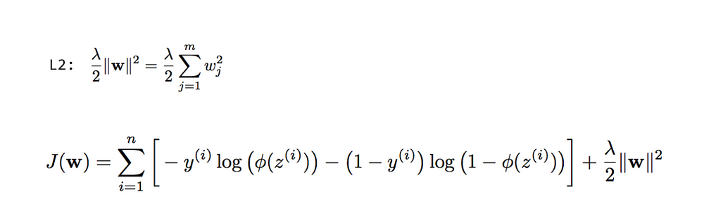
The two common regularization terms, which are added to penalize high coefficients, are the l1 norm or the square of the norm l2 multiplied by ½, which motivates the names L1 and L2 regularization.
The l1 norm is defined as

i.e. the sum of the absolute values of the coefficients, aka the Manhattan distance.
The regularization term for the L2 regularization is defined as

i.e. the sum of the squared of the coefficients, aka the square of the Euclidian distance, multiplied by ½.
Through the parameter λ we can control the impact of the regularization term. Higher values lead to smaller coefficients, but too high values for λ can lead to underfitting.
Support Vector Machine:
The objective of the support vector machine algorithm is to find a hyperplane in an N-dimensional space(N — the number of features) that distinctly classifies the data points.

To separate the two classes of data points, there are many possible hyperplanes that could be chosen. Our objective is to find a plane that has the maximum margin, i.e the maximum distance between data points of both classes. Maximizing the margin distance provides some reinforcement so that future data points can be classified with more confidence.
The objective for an L1-SVM is:
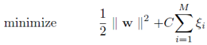
And for an L2-SVM:
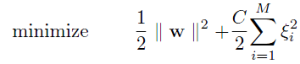
For large values of C, the optimization will choose a smaller-margin hyperplane if that hyperplane does a better job of getting all the training points classified correctly. Conversely, a very small value of C will cause the optimizer to look for a larger-margin separating hyperplane, even if that hyperplane classifies more points.
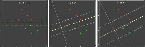
There is no rule of thumb to choose a C value, it totally depends on your testing data.We use gridsearchCV, using which we determine the best value.
Different Regularization techniques in Deep Learning
- L2 and L1 regularization
- Dropout regularization
- Data augmentation
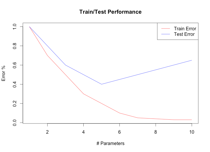
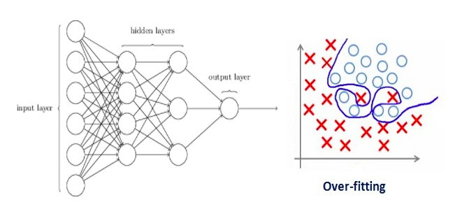
Let’s consider a neural network which is overfitting on the training data as shown in the image below
As we have seen above regularization actually penalizes the weights and in neural nets it penalizes the weight matrices of the nodes.
If our regularization coefficient is so high that some of the weight matrices are nearly equal to zero.
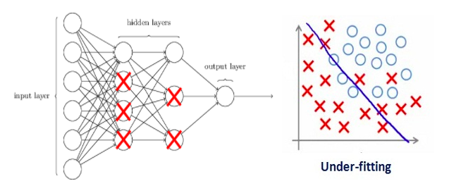
This will result in a much simpler linear network and slight underfitting of the training data.
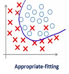
Such a large value of the regularization coefficient is not that useful. We need to optimize the value of regularization coefficient in order to obtain a well-fitted model as shown in the image below.
L2 & L1 regularization:
The general cost function with the regularization term added looks like below,
Cost function = Loss (say, binary cross entropy) + Regularization term
As the cost function must be minimized. By adding the regularization term of the weight matrix and regularization parameters, large weights will be driven down in order to minimize the cost function. Adding the regularization component will drive the values of the weight matrix down. This will effectively decorrelate the neural network.
Recall that we feed the activation function with the following weighted sum:
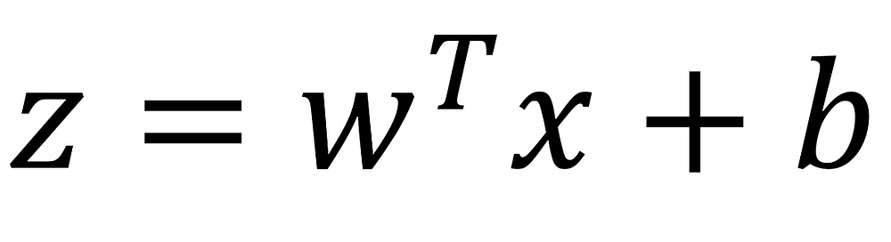
By reducing the values in the weight matrix, z will also be reduced, which in turns decreases the effect of the activation function. Therefore, a less complex function will be fit to the data, effectively reducing overfitting.
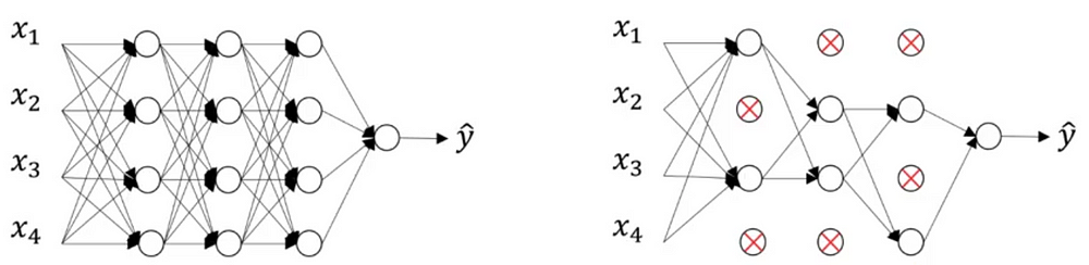
Dropout regularization:
Dropout involves going over all the layers in a neural network and setting probability of keeping a certain nodes or not.
Of course, the input layer and the output layer are kept the same.
The probability of keeping each node is set at random. You only decide of the threshold: a value that will determine if the node is kept or not.
For example, if you set the threshold to 0.7, then there is a probability of 30% that a node will be removed from the network.
Therefore, this will result in a much smaller and simpler neural network, as shown below.
Why dropout works? Dropout means that the neural network cannot rely on any input node, since each have a random probability of being removed. Therefore, the neural network will be reluctant to give high weights to certain features, because they might disappear.
Consequently, the weights are spread across all features, making them smaller. This effectively shrinks the model and regularizes it.
Data Augmentation
The simplest way to reduce overfitting is to increase the size of the training data. In machine learning, we were not able to increase the size of training data as the labeled data was too costly.
Let’s consider we are dealing with images. In this case, there are a few ways of increasing the size of the training data – rotating the image, flipping, scaling, shifting, etc. In the below image, some transformation has been done on the handwritten digits dataset.
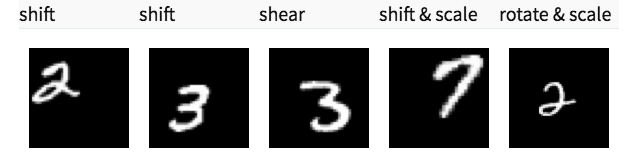
This technique is known as data augmentation. This is usually used to improve the accuracy of the model.
Lets look at the above theory in action:
Here is the code to generate an imbalanced data set where class1 contributes 70% and class2 contributed 30% of the data. First data set forms a moon like shape and the second data set is linearly separable.
import numpy as np
import matplotlib.pyplot as plt
from matplotlib.colors import ListedColormap
from sklearn.model_selection import train_test_split
from sklearn.preprocessing import StandardScaler
from sklearn.datasets import make_moons, make_circles, make_classification
from sklearn.neural_network import MLPClassifier
from sklearn.neighbors import KNeighborsClassifier
from sklearn.svm import SVC
from sklearn.gaussian_process import GaussianProcessClassifier
from sklearn.gaussian_process.kernels import RBF
from sklearn.tree import DecisionTreeClassifier
from sklearn.ensemble import RandomForestClassifier, AdaBoostClassifier
from sklearn.naive_bayes import GaussianNB
from sklearn.discriminant_analysis import QuadraticDiscriminantAnalysis
from imblearn.datasets import make_imbalance
from collections import Counter

h = .02  # step size in the mesh

names = ["RBF SVM", "Logistic Regression",
         "Neural Net"]

classifiers = [
    SVC(gamma=2, C=0.01),
    LogisticRegression(C = 10**15),
    MLPClassifier(hidden_layer_sizes=(200,120,60),alpha=1, max_iter=1000)]

X, y = make_classification(n_samples=300,n_features=2, n_redundant=0, n_informative=2,
                           random_state=1, n_clusters_per_class=1)

rng = np.random.RandomState(2)
X += 2 * rng.uniform(size=X.shape)
linearly_separable = (X, y)

datasets = [make_moons(noise=0.3, random_state=0),
            linearly_separable
            ]

def ratio_func(y, multiplier, minority_class):
    target_stats = Counter(y)
    return {minority_class: int(multiplier * target_stats[minority_class])}

figure = plt.figure(figsize=(27, 9))
i = 1
# iterate over datasets
for ds_cnt, ds in enumerate(datasets):
    # preprocess dataset, split into training and test part
    X, y = ds
    X, y= make_imbalance(X, y, sampling_strategy=ratio_func,
                            **{"multiplier": 0.3,
                               "minority_class": 1})
    X = StandardScaler().fit_transform(X)
    X_train, X_test, y_train, y_test = train_test_split(X, y, test_size=.5, random_state=42)

    x_min, x_max = X[:, 0].min() - .5, X[:, 0].max() + .5
    y_min, y_max = X[:, 1].min() - .5, X[:, 1].max() + .5
    xx, yy = np.meshgrid(np.arange(x_min, x_max, h),
                         np.arange(y_min, y_max, h))
    i += 1

    # iterate over classifiers
    for name, clf in zip(names, classifiers):
        ax = plt.subplot(len(datasets), len(classifiers) + 1, i)
        clf.fit(X_train, y_train)
        score = clf.score(X_test, y_test)

        if hasattr(clf, "decision_function"):
            Z = clf.decision_function(np.c_[xx.ravel(), yy.ravel()])
        else:
            Z = clf.predict_proba(np.c_[xx.ravel(), yy.ravel()])[:, 1]

        Z = clf.predict(np.c_[xx.ravel(), yy.ravel()])
        # Put the result into a color plot
        Z = Z.reshape(xx.shape)
        ax.contourf(xx, yy, Z, alpha=.8)

        # Plot the training points
        ax.scatter(X_train[:, 0], X_train[:, 1], c=y_train,cmap=plt.cm.coolwarm,
                   edgecolors='k')
        # Plot the testing points
        ax.scatter(X_test[:, 0], X_test[:, 1], c=y_test,
                   edgecolors='k',cmap=plt.cm.coolwarm, alpha=0.8)
        ax.set_xlim(xx.min(), xx.max())
        ax.set_ylim(yy.min(), yy.max())
        ax.set_xticks(())
        ax.set_yticks(())
        if ds_cnt == 0:
            ax.set_title(name)
        ax.text(xx.max() - .3, yy.min() + .3, ('%.2f' % score).lstrip('0'),
                size=15, horizontalalignment='right')

        i += 1

plt.tight_layout()
plt.show()
Note that the regularization term is almost made to zero in case of SVM and logistic regression and we have included more weights for MLP.

We could see that all the models are trying to over-fit the majority class1 data points and now let make the below code change to add the regularization term for SVM and logistic regression and change decrease the activation units so the model does not over-fit.
classifiers = [
    SVC(gamma=2, C=10),
    LogisticRegression(C = 10),
    MLPClassifier(hidden_layer_sizes=(60,30,10),alpha=1, max_iter=1000)]
Now the decision surface is more optimal in case of all the models.
