Image forgery detection - vvsnikhil/ML-Blogs GitHub Wiki

Table of Contents:

Introduction
What is Semantic Segmentation?
Understanding the dataset
Understanding Convolution, Max Pooling and Transposed Convolution
UNET Architecture
Building the Model

1. Introduction

The IEEE Information Forensics and Security Technical Committee (IFS-TC) launched a detection and localization forensics challenge, the First Image Forensics Challenge in 2013 to solve this problem. They provided an open dataset of digital images comprising of images taken under different lighting conditions and forged images created using algorithms such as:

Content-Aware Fill and PatchMatch (for copy/pasting)
Content-Aware Healing (for copy/pasting and splicing)
Clone-Stamp (for copy/pasting)
Seam carving (image retargeting)
Inpainting (image reconstruction of damaged parts — a special case of copy/pasting)
Alpha Matting (for splicing)

The challenge consisted of 2 phases.

Phase 1 required participating teams to classify images as forged or pristine (never manipulated)
Phase 2 required them to detect/localize areas of forgery in forged images

This post will be about a deep learning approach to solve the challenge. Everything from data cleaning, pre-processing, CNN architecture to training and evaluation will be elaborated.

2. Custom CNN Architecture

Phase 1 :

Transfer learning

use the weights of a pre-trained model, which probably was trained on a much larger dataset and gave much better results in solving its problem, to solve our problem. In other words, we ‘transfer’ the learning of one model to build ours. In our case, I used the VGG16 and ResNet50 network, trained on ImageNet dataset to vectorize images in our dataset as shown below.

Phase 2:

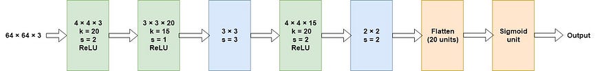
We propose the below two stream Unet model for phase 2. The RGB stream models visual tampering artifacts, such as unusually high contrast along object edges.The noise stream first obtains the noise feature map by passing input RGB image through an SRM filter layer, and leverages the noise features to provide additional evidence for manipulation classification.A bilinear pooling layer after Unet enables the network to combine the spatial co-occurrence features from the two streams. Finally, passing the results through a fully connected layer and a softmax layer, the network produces required mask output.

We would be constructing the below architecture using the Unet model and SRM filters.

3. Dataset

Before going into the dataset overview, the terminology used will be made clear

Fake image: An image that has been manipulated/doctored using the two most common manipulation operations namely: copy/pasting and image splicing.
Pristine image: An image that has not been manipulated except for the resizing needed to bring all images to a standard size as per competition rules.
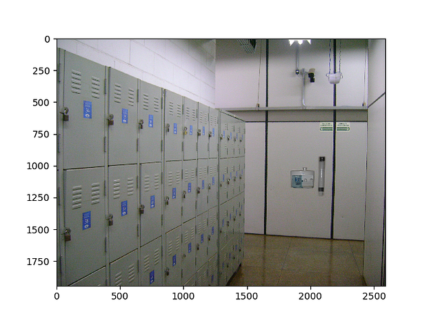
Image splicing: The splicing operations can combine images of people, adding doors to buildings, adding trees and cars to parking lots etc. The spliced images can also contain resulting parts from copy/pasting operations. The image receiving a spliced part is called a “host” image. The parts being spliced together with the host image are referred to as “aliens”.

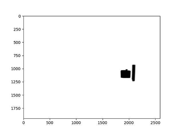
The entire dataset for both the first and second phase can be found here. For this project, we will be using only the train set. It contains 2 directories — one containing fake images and their corresponding masks and the other containing pristine images. Mask of a fake image is a black and white (not grayscale) image describing the spliced area of the fake image. The black pixels in the mask represent the area where manipulation was performed in the source image to get the forged image, specifically it represents the spliced region.

The dataset consists of 1050 pristine and 450 fake images. Color images are usually 3 channel images one channel for each red, green and blue colors, however sometimes the fourth channel for yellow may be present. Images in our dataset are a mix of 1, 3 and 4 channel images. After looking at a couple of 1 channel images i.e. grayscale images, it was evident that these images

were very few in number
were streams of black or blue color

The challenge setters added these images on purpose as they wanted solutions robust to such noise. Although some of the blue images can be images of a clear sky. Hence some of them were included while others discarded as noise. Coming to four channel images — they too didn’t have any useful information. They were simply grids of pixels filled with 0 values. Thus our pristine dataset after cleaning contained about 1025 RGB images. Fake images are a mix of 3 and 4 channel images, however, none of them are noisy. Corresponding masks are a mix of 1, 3 and 4 channel images.Thus our fake image corpus has 450 fakes.

However we will be only using the 450 fake images for phase 2 and we did the train test split to keep 400 fakes for train data and 50 for test data.

4. Understanding Convolution, Max Pooling and Transposed Convolution

Before we dive into the UNET model, it is very important to understand the different operations that are typically used in a Convolutional Network. Please make a note of the terminologies used.

i. Convolution operation

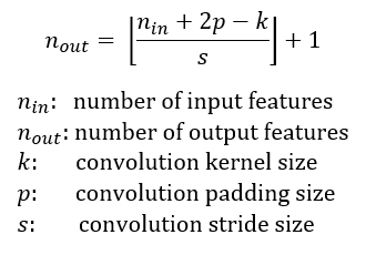
There are two inputs to a convolutional operation i) A 3D volume (input image) of size (nin x nin x channels) ii) A set of ‘k’ filters (also called as kernels or feature extractors) each one of size (f x f x channels), where f is typically 3 or 5. The output of a convolutional operation is also a 3D volume (also called as output image or feature map) of size (nout x nout x k). The relationship between nin and nout is as follows:

Convolution operation can be visualized as follows:

Source: http://cs231n.github.io/convolutional-networks/

In the above GIF, we have an input volume of size 7x7x3. Two filters each of size 3x3x3. Padding =0 and Strides = 2. Hence the output volume is 3x3x2. If you are not comfortable with this arithmetic then you need to first revise the concepts of Convolutional Networks before you continue further.

One important term used frequently is called as the Receptive filed. This is nothing but the region in the input volume that a particular feature extractor (filter) is looking at. In the above GIF, the 3x3 blue region in the input volume that the filter covers at any given instance is the receptive field. This is also sometimes called as the context.

To put in very simple terms, receptive field (context) is the area of the input image that the filter covers at any given point of time.

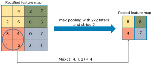
ii) Max pooling operation In simple words, the function of pooling is to reduce the size of the feature map so that we have fewer parameters in the network. For example:

Source: https://www.quora.com/What-is-max-pooling-in-convolutional-neural-networks#

Basically from every 2x2 block of the input feature map, we select the maximum pixel value and thus obtain a pooled feature map. Note that the size of the filter and strides are two important hyper-parameters in the max pooling operation. The idea is to retain only the important features (max valued pixels) from each region and throw away the information which is not important. By important, I mean that information which best describes the context of the image.

A very important point to note here is that both convolution operation and specially the pooling operation reduce the size of the image. This is called as down sampling. In the above example, the size of the image before pooling is 4x4 and after pooling is 2x2. In fact down sampling basically means converting a high resolution image to a low resolution image.

Thus before pooling, the information which was present in a 4x4 image, after pooling, (almost) the same information is now present in a 2x2 image.

Now when we apply the convolution operation again, the filters in the next layer will be able to see larger context, i.e. as we go deeper into the network, the size of the image reduces however the receptive field increases. For example, below vgg16 architecture:

VGG16 Notice that in a typical convolutional network, the height and width of the image gradually reduces (down sampling, because of pooling) which helps the filters in the deeper layers to focus on a larger receptive field (context). However the number of channels/depth (number of filters used) gradually increase which helps to extract more complex features from the image.

Intuitively we can make the following conclusion of the pooling operation. By down sampling, the model better understands “WHAT” is present in the image, but it loses the information of “WHERE” it is present.

iii) Need for up sampling As stated previously, the output of semantic segmentation is not just a class label or some bounding box parameters. In-fact the output is a complete high resolution image in which all the pixels are classified. Thus if we use a regular convolutional network with pooling layers and dense layers, we will lose the “WHERE” information and only retain the “WHAT” information which is not what we want. In case of segmentation we need both “WHAT” as well as “WHERE” information.

Hence there is a need to up sample the image, i.e. convert a low resolution image to a high resolution image to recover the “WHERE” information.

In the literature, there are many techniques to up sample an image. Some of them are bi-linear interpolation, cubic interpolation, nearest neighbor interpolation, unpooling, transposed convolution, etc. However in most state of the art networks, transposed convolution is the preferred choice for up sampling an image.

iv) Transposed Convolution Transposed convolution (sometimes also called as deconvolution or fractionally strided convolution) is a technique to perform up sampling of an image with learn able parameters

On a high level, transposed convolution is exactly the opposite process of a normal convolution i.e., the input volume is a low resolution image and the output volume is a high resolution image.

5. UNET Architecture

The UNETwas developed by Olaf Ronneberger et al. for Bio Medical Image Segmentation. The architecture contains two paths. First path is the contraction path (also called as the encoder) which is used to capture the context in the image. The encoder is just a traditional stack of convolutional and max pooling layers. The second path is the symmetric expanding path (also called as the decoder) which is used to enable precise localization using transposed convolutions. Thus it is an end-to-end fully convolutional network (FCN), i.e. it only contains Convolutional layers and does not contain any Dense layer because of which it can accept image of any size.

In the original paper, the UNET is described as follows:

I will try to describe this architecture much more intuitively. Note that in the original paper, the size of the input image is 572x572x3, however, we will use input image of size 512x512x3. Hence the size at various locations will differ from that in the original paper but the core components remain the same. Below is the detailed explanation of the architecture:

This is what gives the architecture a symmetric U-shape, hence the name UNET
On a high level, we have the following relationship: Input (512x512x3) => Encoder =>(8x8x256) => Decoder =>Ouput (512x512x1)

6. Building the model

Phase1:

Apart from VGG16 we also tried bottleneck features from ResNet50 and VGG19 models pre-trained on Image-Net dataset. Features from ResNet50 outperform VGG16. VGG16 has given the below test accuracy.

Validation accuracy : 93.5%, Validation loss : 0.35

resnet_model=ResNet50(weights='imagenet', include_top=False, input_shape=(64, 64, 3))

model_aug=Sequential()
model_aug.add(resnet_model)

top_model=Sequential()
top_model.add(Flatten(input_shape=(2, 2, 2048)))

top_model.add(Dense(64, activation='relu'))
model_aug.add(Dropout(0.2))
top_model.add(Dense(1, activation='sigmoid'))

model_aug.add(top_model)

for layer in model_aug.layers[0].layers[:171]:
    layer.trainable=False

model_aug.load_weights('fine_tuned_resnet_adam_weights.h5')

model_aug.compile(loss='binary_crossentropy', optimizer=keras.optimizers.Adam(lr=1e-3), metrics=['accuracy'])

Results: The fine-tuned ResNet50 model was used to predict labels for these patches and gave the following results.

Validation accuracy : 94.5%, Validation loss : 0.22

Phase2:

Now that we got an idea of how we build a Unet model, we will be using the below SRM filter to create the noise images.

Below is the Keras code to construct the proposed model

q = [4.0, 12.0, 2.0]
filter1 = [[0, 0, 0, 0, 0],
           [0, -1, 2, -1, 0],
           [0, 2, -4, 2, 0],
           [0, -1, 2, -1, 0],
           [0, 0, 0, 0, 0]]
filter2 = [[-1, 2, -2, 2, -1],
           [2, -6, 8, -6, 2],
           [-2, 8, -12, 8, -2],
           [2, -6, 8, -6, 2],
           [-1, 2, -2, 2, -1]]
filter3 = [[0, 0, 0, 0, 0],
           [0, 0, 0, 0, 0],
           [0, 1, -2, 1, 0],
           [0, 0, 0, 0, 0],
           [0, 0, 0, 0, 0]]


filter1 = np.asarray(filter1, dtype=float) / q[0]
filter2 = np.asarray(filter2, dtype=float) / q[1]
filter3 = np.asarray(filter3, dtype=float) / q[2]
    
filters = filter1+filter2+filter3

for x in fakes:
    image = imread(fake_path+x)
    processed_image = cv2.filter2D(image,-1,filters)
    plt.imsave(x,processed_image)

batch_size = 1
max_epochs = 100
input_size = 512

def conv2d_block(input_dim, n_filters, kernel_size=3, batchnorm=True):
    x = Conv2D(filters=n_filters, kernel_size=(kernel_size, kernel_size), kernel_initializer="he_normal",padding="same") (input_dim)
    x = BatchNormalization()(x)
    x = Activation("relu")(x)
    x = Conv2D(filters=n_filters, kernel_size=(kernel_size, kernel_size), kernel_initializer="he_normal",padding="same")(x)
    x = BatchNormalization()(x)
    final_block = Activation("relu")(x)
    return final_block

input_img = Input((512, 512, 3), name='img1')
n_filters=16
batchnorm=True
dropout=0.5
# contracting path
c1 = conv2d_block(input_img, n_filters=n_filters*1, kernel_size=3, batchnorm=batchnorm)
p1 = MaxPooling2D((2, 2)) (c1)
p1 = Dropout(dropout*0.5)(p1)
c2 = conv2d_block(p1, n_filters=n_filters*2, kernel_size=3, batchnorm=batchnorm)
p2 = MaxPooling2D((2, 2)) (c2)
p2 = Dropout(dropout)(p2)
c3 = conv2d_block(p2, n_filters=n_filters*4, kernel_size=3, batchnorm=batchnorm)
p3 = MaxPooling2D((2, 2)) (c3)
p3 = Dropout(dropout)(p3)
c4 = conv2d_block(p3, n_filters=n_filters*8, kernel_size=3, batchnorm=batchnorm)
p4 = MaxPooling2D(pool_size=(2, 2)) (c4)
p4 = Dropout(dropout)(p4)
c5 = conv2d_block(p4, n_filters=n_filters*16, kernel_size=3, batchnorm=batchnorm)
#Expanding path
u6 = Conv2DTranspose(n_filters*8, (3, 3), strides=(2, 2), padding='same') (c5)
#skip_connections
u6 = concatenate([u6, c4])
u6 = Dropout(dropout)(u6)
c6 = conv2d_block(u6, n_filters=n_filters*8, kernel_size=3, batchnorm=batchnorm)
u7 = Conv2DTranspose(n_filters*4, (3, 3), strides=(2, 2), padding='same') (c6)
u7 = concatenate([u7, c3])
u7 = Dropout(dropout)(u7)
c7 = conv2d_block(u7, n_filters=n_filters*4, kernel_size=3, batchnorm=batchnorm)
u8 = Conv2DTranspose(n_filters*2, (3, 3), strides=(2, 2), padding='same') (c7)
u8 = concatenate([u8, c2])
u8 = Dropout(dropout)(u8)
c8 = conv2d_block(u8, n_filters=n_filters*2, kernel_size=3, batchnorm=batchnorm)
u9 = Conv2DTranspose(n_filters*1, (3, 3), strides=(2, 2), padding='same') (c8)
u9 = concatenate([u9, c1], axis=3)
u9 = Dropout(dropout)(u9)
c9 = conv2d_block(u9, n_filters=n_filters*1, kernel_size=3, batchnorm=batchnorm)

output = Conv2D(3, (1, 1), activation='sigmoid') (c9)
#model1 = Model(inputs=[input_img], outputs=[outputs])


input_img_filter = Input((512, 512, 3), name='img2')
n_filters=16
batchnorm=True
dropout=0.5

# contracting path
c1 = conv2d_block(input_img_filter, n_filters=n_filters*1, kernel_size=3, batchnorm=batchnorm)
p1 = MaxPooling2D((2, 2)) (c1)
p1 = Dropout(dropout*0.5)(p1)
c2 = conv2d_block(p1, n_filters=n_filters*2, kernel_size=3, batchnorm=batchnorm)
p2 = MaxPooling2D((2, 2)) (c2)
p2 = Dropout(dropout)(p2)
c3 = conv2d_block(p2, n_filters=n_filters*4, kernel_size=3, batchnorm=batchnorm)
p3 = MaxPooling2D((2, 2)) (c3)
p3 = Dropout(dropout)(p3)
c4 = conv2d_block(p3, n_filters=n_filters*8, kernel_size=3, batchnorm=batchnorm)
p4 = MaxPooling2D(pool_size=(2, 2)) (c4)
p4 = Dropout(dropout)(p4)
c5 = conv2d_block(p4, n_filters=n_filters*16, kernel_size=3, batchnorm=batchnorm)
#Expanding path
u6 = Conv2DTranspose(n_filters*8, (3, 3), strides=(2, 2), padding='same') (c5)
#skip_connections
u6 = concatenate([u6, c4])
u6 = Dropout(dropout)(u6)
c6 = conv2d_block(u6, n_filters=n_filters*8, kernel_size=3, batchnorm=batchnorm)
u7 = Conv2DTranspose(n_filters*4, (3, 3), strides=(2, 2), padding='same') (c6)
u7 = concatenate([u7, c3])
u7 = Dropout(dropout)(u7)
c7 = conv2d_block(u7, n_filters=n_filters*4, kernel_size=3, batchnorm=batchnorm)
u8 = Conv2DTranspose(n_filters*2, (3, 3), strides=(2, 2), padding='same') (c7)
u8 = concatenate([u8, c2])
u8 = Dropout(dropout)(u8)
c8 = conv2d_block(u8, n_filters=n_filters*2, kernel_size=3, batchnorm=batchnorm)
u9 = Conv2DTranspose(n_filters*1, (3, 3), strides=(2, 2), padding='same') (c8)
u9 = concatenate([u9, c1], axis=3)
u9 = Dropout(dropout)(u9)
c9 = conv2d_block(u9, n_filters=n_filters*1, kernel_size=3, batchnorm=batchnorm)

output_filter = Conv2D(3, (1, 1), activation='sigmoid') (c9)

combined = concatenate([output, output_filter])
outputs = Conv2D(1, (1, 1), activation='sigmoid') (combined)

model = Model(inputs=[input_img,input_img_filter], outputs=[outputs])

Here are the results from the above model

Predicted Mask:

Actual Mask:

Report:

ELA+UNET
ELA + SRM Filter
Fakes+SRM Filter

Out of the above three we have used data augmentations for 1 and 2 unfortunately they have not performed as expected. Model 3 Fake + SRM filter has done reasonably well.

There is a lot of scope to improve the performance for phase 2 by using data augmentations and also including the pristine images in train data set with default mask.

Sources: