1 Putting it all together

1.1 Putting it all together

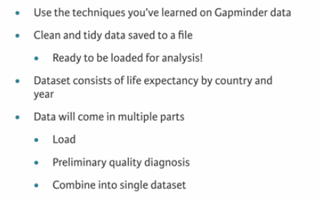
1.2 Useful methods

1.3 Data quality

1.4 combining data

1.5 Example 1: Exploratory analysis

Whenever you obtain a new dataset, your first task should always be to do some exploratory analysis to get a better understanding of the data and diagnose it for any potential issues.

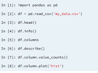
The Gapminder data for the 19th century has been loaded into a DataFrame called g1800s. In the IPython Shell, use pandas methods such as .head(), .info(), and .describe(), and DataFrame attributes like .columns and .shape to explore it.

Use the information that you acquire from your exploratory analysis to choose the true statement from the options provided below.

1.6 Example 2: Visualizing your data

Since 1800, life expectancy around the globe has been steadily going up. You would expect the Gapminder data to confirm this.

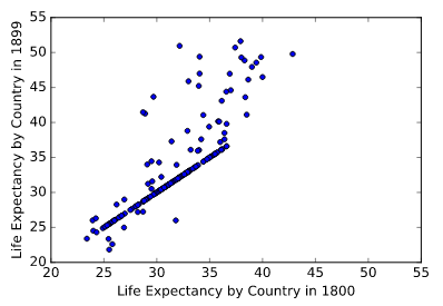
The DataFrame g1800s has been pre-loaded. Your job in this exercise is to create a scatter plot with life expectancy in '1800' on the x-axis and life expectancy in '1899' on the y-axis.

Here, the goal is to visually check the data for insights as well as errors. When looking at the plot, pay attention to whether the scatter plot takes the form of a diagonal line, and which points fall below or above the diagonal line. This will inform how life expectancy in 1899 changed (or did not change) compared to 1800 for different countries. If points fall on a diagonal line, it means that life expectancy remained the same!

# Import matplotlib.pyplot
import matplotlib.pyplot as plt

# Create the scatter plot
g1800s.plot(kind='scatter', x='1800', y='1899')

# Specify axis labels
plt.xlabel('Life Expectancy by Country in 1800')
plt.ylabel('Life Expectancy by Country in 1899')

# Specify axis limits
plt.xlim(20, 55)
plt.ylim(20, 55)

# Display the plot
plt.show()

RESULT:

Excellent work! As you can see, there are a surprising number of countries that fall on the diagonal line. In fact, examining the DataFrame reveals that the life expectancy for 140 of the 260 countries did not change at all in the 19th century! This is possibly a result of not having access to the data for all the years back then. In this way, visualizing your data can help you uncover insights as well as diagnose it for errors.

1.7 Example 3: Thinking about the question at hand

LINK

Since you are given life expectancy level data by country and year, you could ask questions about how much the average life expectancy changes over each year.

Before continuing, however, it's important to make sure that the following assumptions about the data are true:

* `'Life expectancy'` is the first column (index `0`) of the DataFrame.
* The other columns contain either null or numeric values.
* The numeric values are all greater than or equal to 0.
* There is only one instance of each country.

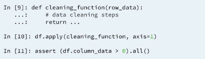
You can write a function that you can apply over the entire DataFrame to verify some of these assumptions. Note that spending the time to write such a script will help you when working with other datasets as well.

def check_null_or_valid(row_data):
    """Function that takes a row of data,
    drops all missing values,
    and checks if all remaining values are greater than or equal to 0
    """
    no_na = row_data.dropna()[1:-1] # 1800  and 1899  excluded (1801 - 1898 are included)  . i        mean after dropna we only take  1801 - 1898 for make theme numeric.

    numeric = pd.to_numeric(no_na, errors='coerce') # numeric <class 'pandas.core.series.Series'>
    ge0 = numeric >= 0 # ge0 is  <class 'pandas.core.series.Series'> of bool value
    return ge0

# Check whether the first column is 'Life expectancy'
assert g1800s.columns[0] == 'Life expectancy'

# Check whether the values in the row are valid
assert g1800s.iloc[:, 1:].apply(check_null_or_valid, axis=1).all().all() # exclude the 'Life expextancy column'

# Check that there is only one instance of each country
assert g1800s['Life expectancy'].value_counts()[0] == 1

1.8 Assembling your data

Here, three DataFrames have been pre-loaded: g1800s, g1900s, and g2000s. These contain the Gapminder life expectancy data for, respectively, the 19th century, the 20th century, and the 21st century.

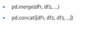
Your task in this exercise is to concatenate them into a single DataFrame called gapminder. This is a row-wise concatenation, similar to how you concatenated the monthly Uber datasets in Chapter 3.

# Concatenate the DataFrames row-wise
gapminder = pd.concat([g1800s, g1900s, g2000s])

# Print the shape of gapminder
print(gapminder.shape)

# Print the head of gapminder
print(gapminder.head())

2 Initial impressions of the data

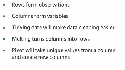
2.1 principles of tidy data

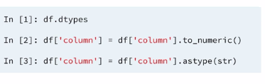
2.2 checking data types

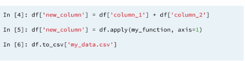
2.3 Additional calculations and saving your data

2.4 Example 4

Now that you have all the data combined into a single DataFrame, the next step is to reshape it into a tidy data format.

Currently, the gapminder DataFrame has a separate column for each year. What you want instead is a single column that contains the year, and a single column that represents the average life expectancy for each year and country. By having year in its own column, you can use it as a predictor variable in a later analysis.

You can convert the DataFrame into the desired tidy format by melting it.

# Melt gapminder: gapminder_melt
gapminder_melt = pd.melt(frame=gapminder,  id_vars='Life expectancy')

# Rename the columns
gapminder_melt.columns = ['country', 'year', 'life_expectancy']

# Print the head of gapminder_melt
print(gapminder_melt.head())

2.5 Example 5 : Checking the data types

Now that your data is in the proper shape, you need to ensure that the columns are of the proper data type. That is, you need to ensure that country is of type object, year is of type int64, and life_expectancy is of type float64.

The tidy DataFrame has been pre-loaded as gapminder. Explore it in the IPython Shell using the .info() method. Notice that the column 'year' is of type object. This is incorrect, so you'll need to use the pd.to_numeric() function to convert it to a numeric data type.

NumPy and pandas have been pre-imported as np and pd.

# Convert the year column to numeric
gapminder.year = pd.to_numeric(gapminder.year, errors='coerce')

# Test if country is of type object
assert gapminder.country.dtypes == np.object

# Test if year is of type int64
assert gapminder.year.dtypes == np.int64

# Test if life_expectancy is of type float64
assert gapminder.life_expectancy.dtypes == np.float64

2.6 Example 6 : Looking at country spellings

Having tidied your DataFrame and checked the data types, your next task in the data cleaning process is to look at the 'country' column to see if there are any special or invalid characters you may need to deal with.

It is reasonable to assume that country names will contain:

* The set of lower and upper case letters.
* Whitespace between words.
* Periods for any abbreviations.

To confirm that this is the case, you can leverage the power of regular expressions again. For common operations like this, Python has a built-in string method - str.contains() - which takes a regular expression pattern, and applies it to the Series, returning True if there is a match, and False otherwise.

Since here you want to find the values that do not match, you have to invert the boolean, which can be done using ~. This Boolean series can then be used to get the Series of countries that have invalid names.

# Create the series of countries: countries
countries = gapminder['country']

# Drop all the duplicates from countries
countries = countries.drop_duplicates()

# Write the regular expression: pattern
pattern = '^[A-Za-z\.\s]*$'

# Create the Boolean vector: mask
mask = countries.str.contains(pattern)

# Invert the mask: mask_inverse
mask_inverse = ~ mask

# Subset countries using mask_inverse: invalid_countries
invalid_countries = countries.loc[mask_inverse]

# Print invalid_countries
print(invalid_countries)

2.7 Example 7 : More data cleaning and processing

It's now time to deal with the missing data. There are several strategies for this: You can drop them, fill them in using the mean of the column or row that the missing value is in (also known as imputation), or, if you are dealing with time series data, use a forward fill or backward fill, in which you replace missing values in a column with the most recent known value in the column. See pandas Foundations for more on forward fill and backward fill.

In general, it is not the best idea to drop missing values, because in doing so you may end up throwing away useful information. In this data, the missing values refer to years where no estimate for life expectancy is available for a given country. You could fill in, or guess what these life expectancies could be by looking at the average life expectancies for other countries in that year, for example. Whichever strategy you go with, it is important to carefully consider all options and understand how they will affect your data.

In this exercise, you'll practice dropping missing values. Your job is to drop all the rows that have NaN in the life_expectancy column. Before doing so, it would be valuable to use assert statements to confirm that year and country do not have any missing values.

Begin by printing the shape of gapminder in the IPython Shell prior to dropping the missing values. Complete the exercise to find out what its shape will be after dropping the missing values!

Instructions:

• Assert that country and year do not contain any missing values. The first assert statement has been written for you. Note the chaining of the .all() method to pd.notnull() to confirm that all values in the column are not null.
• Drop the rows in the data where any observation in life_expectancy is missing. As you confirmed that country and year don't have missing values, you can use the .dropna() method on the entire gapminder DataFrame, because any missing values would have to be in the life_expectancy column. The .dropna() method has the default keyword arguments axis=0 and how='any', which specify that rows with any missing values should be dropped. *Print the shape of gapminder.

# Assert that country does not contain any missing values
assert pd.notnull(gapminder.country).all()

# Assert that year does not contain any missing values
assert pd.notnull(gapminder.year).all()

# Drop the missing values
gapminder = gapminder.dropna(axis=0, how='any')

# Print the shape of gapminder
print(gapminder.shape)

Results:

Great work! After dropping the missing values from 'life_expectancy', the number of rows in the DataFrame has gone down from 169260 to 43857. In general, you should avoid dropping too much of your data, but if there is no reasonable way to fill in or impute missing values, then dropping the missing data may be the best solution.

2.8 Example 8 : More data cleaning and processing

LINK

Now that you have a clean and tidy dataset, you can do a bit of visualization and aggregation. In this exercise, you'll begin by creating a histogram of the life_expectancy column. You should not get any values under 0 and you should see something reasonable on the higher end of the life_expectancy age range.

Your next task is to investigate how average life expectancy changed over the years. To do this, you need to subset the data by each year, get the life_expectancy column from each subset, and take an average of the values. You can achieve this using the .groupby() method. This .groupby() method is covered in greater depth in Manipulating DataFrames with pandas.

Finally, you can save your tidy and summarized DataFrame to a file using the .to_csv() method.

Matplotlib and pandas have been pre-imported as plt and pd. Go for it!

INSTRUCTIONS :

• Create a histogram of the life_expectancy column using the .plot() method of gapminder. Specify kind='hist'.
• Group gapminder by 'year' and aggregate 'life_expectancy' by the mean. To do this: Use the .groupby() method on gapminder with 'year' as the argument. Then select 'life_expectancy' and chain the .mean() method to it.
• Print the head and tail of gapminder_agg. This has been done for you.
• Create a line plot of average life expectancy per year by using the .plot() method (without any arguments) on gapminder_agg. Save gapminder and gapminder_agg to csv files called 'gapminder.csv' and 'gapminder_agg.csv', respectively, using the .to_csv() method.

# Add first subplot
plt.subplot(2, 1, 1) 

# Create a histogram of life_expectancy
gapminder.life_expectancy.plot(kind='hist')

# Group gapminder: gapminder_agg
gapminder_agg = gapminder.groupby('year')['life_expectancy'].mean()
print(gapminder.groupby('year'))

# Print the head of gapminder_agg
print(gapminder_agg.head())

# Print the tail of gapminder_agg
print(gapminder_agg.tail())

# Add second subplot
plt.subplot(2, 1, 2)

# Create a line plot of life expectancy per year
gapminder_agg.plot()

# Add title and specify axis labels
plt.title('Life expectancy over the years')
plt.ylabel('Life expectancy')
plt.xlabel('Year')

# Display the plots
plt.tight_layout()
plt.show()

# Save both DataFrames to csv files
gapminder.to_csv('gapminder.csv')
gapminder_agg.to_csv('gapminder_agg.csv')

**Results: **

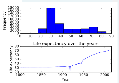
Amazing work! You've stepped through each stage of the data cleaning process and your data is now ready for serious analysis! Looking at the line plot, it seems like life expectancy has, as expected, increased over the years. There is a surprising dip around 1920 that may be worth further investigation!

3 Final thoughts

3.1 You have learned how too ...

4 Cleaning data Steps

Exploratory analysis Visualizing your data Thinking about the question at hand Assembling your data Reshaping your data Checking the data types Looking at country spellings More data cleaning and processing Wrapping up