1 Case Study - Summer Olympics

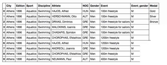
1.1 Olympic medals dataset

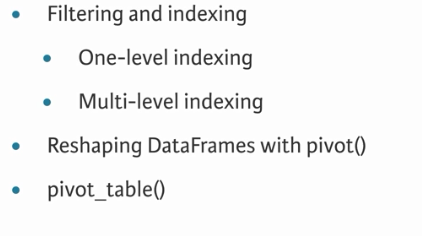
1.2 Reminder: indexing & pivoting

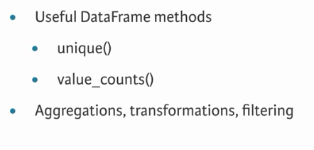
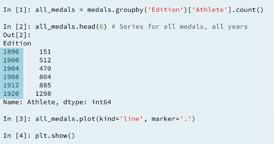
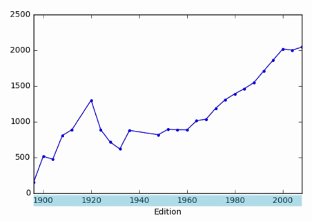
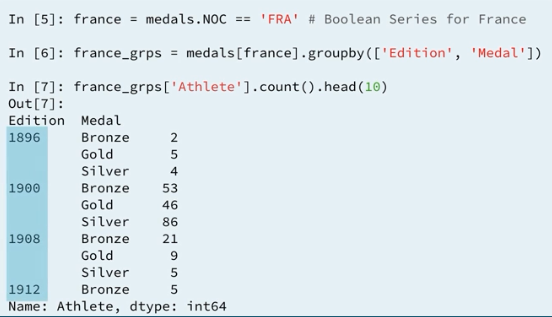
1.3 Reminder: groupby

1.4 Example 1 : Using .value_counts() for ranking

For this exercise, you will use the pandas Series method .value_counts() to determine the top 15 countries ranked by total number of medals.

Notice that .value_counts() sorts by values by default. The result is returned as a Series of counts indexed by unique entries from the original Series with values (counts) ranked in descending order.

The DataFrame has been pre-loaded for you as medals.

# Select the 'NOC' column of medals: country_names
country_names = medals['NOC']

# Count the number of medals won by each country: medal_counts
medal_counts = country_names.value_counts()

# Print top 15 countries ranked by medals
print(medal_counts.head(15))

1.5 Example 2 : Using .pivot_table() to count medals by type

Using .pivot_table() to count medals by type**

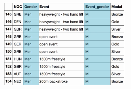
2 Understanding the column labels

2.1 "Gender" and "Event gender"

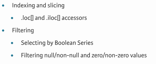
2.1 Reminder: slicing & filtering

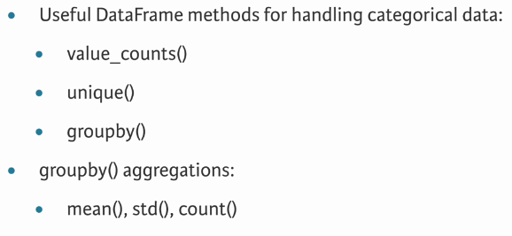
2.2 Reminder: Handling categorical data

3 Constructing alternative country rankings

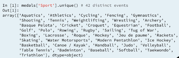
3.1 Counting distinct events

3.2 Ranking of distinct events

3.3 Two new dataframe methods

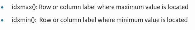
3.4 idxmax() Example

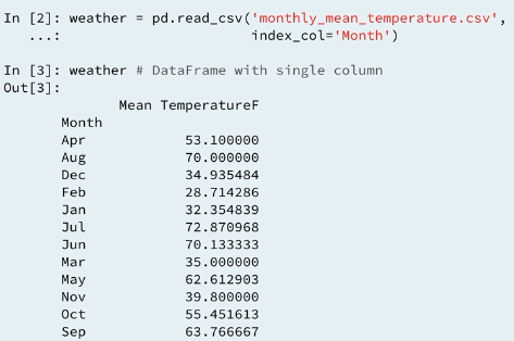
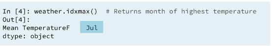
3.5 Using idxmax()

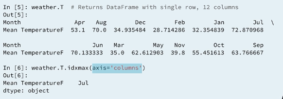
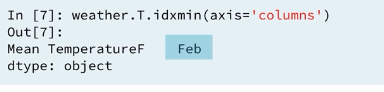
3.6 Using idxmax() along columns

3.7 Using idxmin()

3.8 Example 3 : Using .nunique() to rank by distinct sports

Counting USA vs. USSR Cold War Olympic Sports

See the use of isin and nunique.

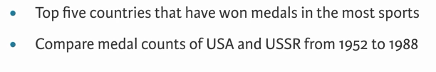
The Olympic competitions between 1952 and 1988 took place during the height of the Cold War between the United States of America (USA) & the Union of Soviet Socialist Republics (USSR). Your goal in this exercise is to aggregate the number of distinct sports in which the USA and the USSR won medals during the Cold War years.

The construction is mostly the same as in the preceding exercise. There is an additional filtering stage beforehand in which you reduce the original DataFrame medals by extracting data from the Cold War period that applies only to the US or to the USSR. The relevant country codes in the DataFrame, which has been pre-loaded as medals, are 'USA' & 'URS'.

# Extract all rows for which the 'Edition' is between 1952 & 1988: during_cold_war
during_cold_war =(medals.Edition>=1952) & (medals.Edition<=1988)

# Extract rows for which 'NOC' is either 'USA' or 'URS': is_usa_urs
is_usa_urs = medals.NOC.isin(['USA', 'URS'])

# Use during_cold_war and is_usa_urs to create the DataFrame: cold_war_medals
cold_war_medals = medals.loc[during_cold_war & is_usa_urs]

# Group cold_war_medals by 'NOC'
country_grouped = cold_war_medals.groupby('NOC')

# Create Nsports
Nsports = country_grouped['Sport'].nunique().sort_values(ascending=False)

# Print Nsports
print(Nsports)

3.9 Example 4 : Counting USA vs. USSR Cold War Olympic Medals

PLAY BY PLAY

# Create the pivot table: medals_won_by_country
medals_won_by_country = medals.pivot_table(index='Edition', columns='NOC', values='Athlete', aggfunc='count')

SEEMS LIKE.... Here is you use the pivot_table without the aggfunc then you will get an error becaue Athlete column is string type and defalut same row paile average ta count kore but jeheu string ar average hoi na tai error dei.

Counting USA vs. USSR Cold War Olympic Medals

4 Reshaping DataFrames for visualization

4.1 Reminder: Plotting DataFrames

4.2 Plotting Dataframes

4.3 Grouping the data

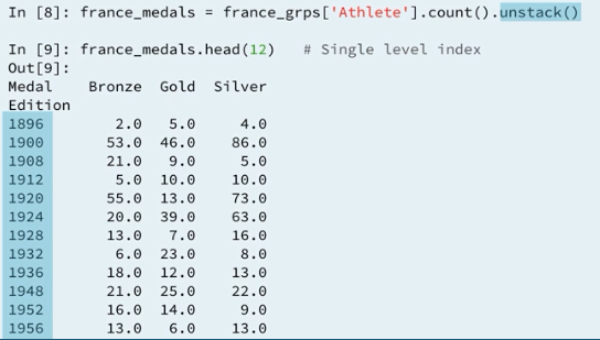
Plotting tools like matplotlib works best with one level index. The Tool you want here is unstack to unpack the multi index.

4.4 Reshaping the data

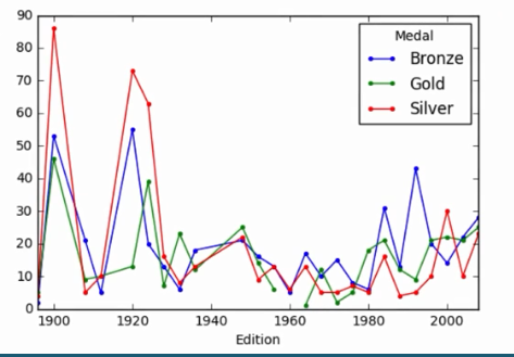
4.5 Plotting the result

4.6 Example 5 : Visualizing USA Medal Counts by Edition: Line Plot

Visualizing USA Medal Counts by Edition: Line Plot

Your job in this exercise is to visualize the medal counts by 'Edition' for the USA. The DataFrame has been pre-loaded for you as medals.

# Create the DataFrame: usa
usa = medals.loc[medals.NOC == 'USA']

# Group usa by ['Edition', 'Medal'] and aggregate over 'Athlete'
usa_medals_by_year =usa.groupby(['Edition', 'Medal'])['Athlete'].count()

# Reshape usa_medals_by_year by unstacking
usa_medals_by_year = usa_medals_by_year.unstack(level='Medal')

# Plot the DataFrame usa_medals_by_year
usa_medals_by_year.plot()
plt.show()

example

You may have noticed that the medals are ordered according to a lexicographic (dictionary) ordering: Bronze < Gold < Silver. However, you would prefer an ordering consistent with the Olympic rules: Bronze < Silver < Gold.

You can achieve this using Categorical types. In this final exercise, after redefining the 'Medal' column of the DataFrame medals, you will repeat the area plot from the previous exercise to see the new ordering.

# Redefine 'Medal' as an ordered categorical
medals.Medal = pd.Categorical(values = medals.Medal, categories=['Bronze', 'Silver', 'Gold'], ordered=True)

# Create the DataFrame: usa
usa = medals[medals.NOC == 'USA']

# Group usa by 'Edition', 'Medal', and 'Athlete'
usa_medals_by_year = usa.groupby(['Edition', 'Medal'])['Athlete'].count()

# Reshape usa_medals_by_year by unstacking
usa_medals_by_year = usa_medals_by_year.unstack(level='Medal')

print(usa_medals_by_year)

# Create an area plot of usa_medals_by_year
usa_medals_by_year.plot.area()
plt.show()

5 Congetulations

5.1 You can now...