For more about groupby

1 Categoricals and groupby

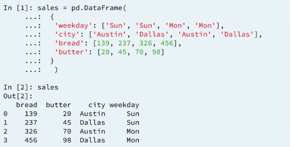
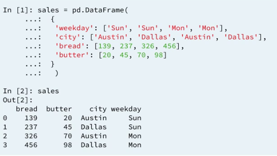
1.1 Sales data

1.2 Boolean filter and count

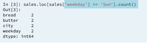
Here we have to know that Sun exist in the column.

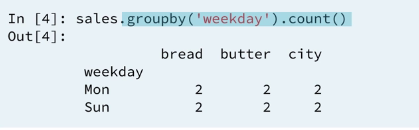
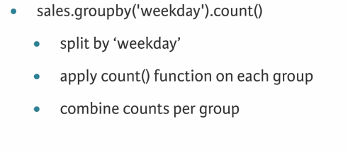
1.3 Groupby and count

1.4 Split-apply-combine

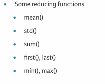
1.5 Aggregation/Reduction

Pandas groupby works with many statistical reduction we have seen so far.

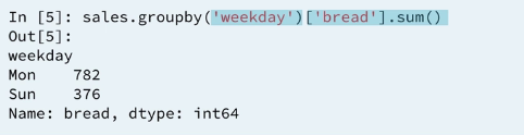
1.6 Groupby and sum

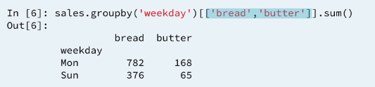
1.7 Groupby and sum : multiple columns

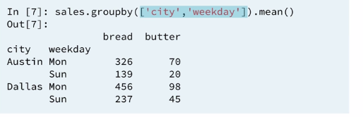
1.8 Groupby and mean: multi-level index**

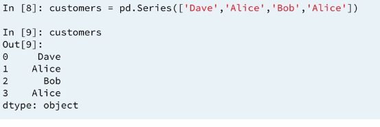
so far we have used column names only within the group by. In fact we can use any pandas series with the same index values. for instance:

1.9 Customers

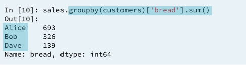
1.10 Groupby and sum : by series**

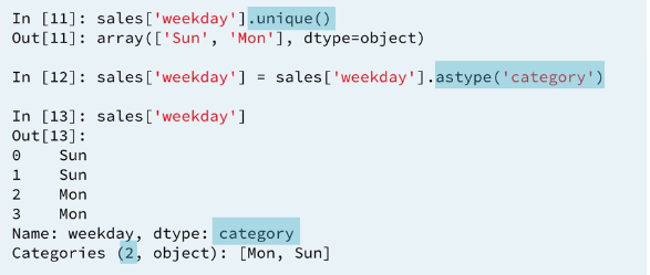
1.11 Categorical data

ordered categorical**

1.12 Example 1 : Grouping by another series**

Grouping by another series

2 Groupby and aggregation

2.1 sales data

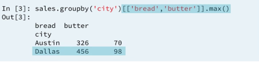
2.2 Review: groupby

2.3 Multiple aggregations

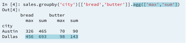
The result is displayed using a multi label index for the columns.

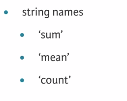
2.4 Aggregation functions

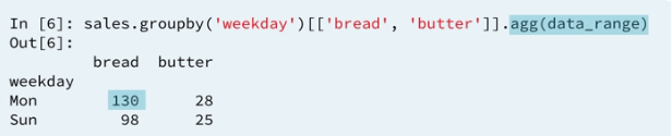
2.5 Custom aggregation

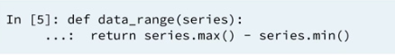
This is an aggregation because it receives a series and returns a single number.

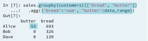
2.6 Custom aggregation: dictionaries

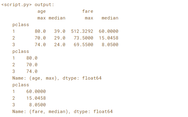
2.7 Example 2: Computing multiple aggregates of multiple columns

Link

The .agg() method can be used with a tuple or list of aggregations as input. When applying multiple aggregations on multiple columns, the aggregated DataFrame has a multi-level column index.

In this exercise, you're going to group passengers on the Titanic by 'pclass' and aggregate the 'age' and 'fare' columns by the functions 'max' and 'median'. You'll then use multi-level selection to find the oldest passenger per class and the median fare price per class.

The DataFrame has been pre-loaded as titanic.

# Group titanic by 'pclass': by_class
by_class = titanic.groupby('pclass')

# Select 'age' and 'fare'
by_class_sub = by_class['age','fare'](/upalr/Python-camp/wiki/'age','fare')

# Aggregate by_class_sub by 'max' and 'median': aggregated
aggregated = by_class_sub.agg(['max', 'median'])

print(aggregated)

# Print the maximum age in each class
print(aggregated.loc[:, ('age','max')])

# Print the median fare in each class
print(aggregated.loc[:, ('fare','median')])

2.8 Example 3 : Aggregating on index levels**/fields

Link

If you have a DataFrame with a multi-level row index, the individual levels can be used to perform the groupby. This allows advanced aggregation techniques to be applied along one or more levels in the index and across one or more columns.

In this exercise you'll use the full Gapminder dataset which contains yearly values of life expectancy, population, child mortality (per 1,000) and per capita gross domestic product (GDP) for every country in the world from 1964 to 2013.

Your job is to create a multi-level DataFrame of the columns 'Year', 'Region' and 'Country'. Next you'll group the DataFrame by the 'Year' and 'Region' levels. Finally, you'll apply a dictionary aggregation to compute the total population, spread of per capita GDP values and average child mortality rate.

The Gapminder CSV file is is available as 'gapminder.csv'.

# Read the CSV file into a DataFrame and sort the index: gapminder
gapminder = pd.read_csv('gapminder.csv', index_col=['Year','region','Country']).sort_index()

# Group gapminder by 'Year' and 'region': by_year_region
by_year_region = gapminder.groupby(level=['Year', 'region'])

# Define the function to compute spread: spread
def spread(series):
    return series.max() - series.min()

# Create the dictionary: aggregator
aggregator = {'population':'sum', 'child_mortality':'mean', 'gdp':spread}

# Aggregate by_year_region using the dictionary: aggregated
aggregated = by_year_region.agg(aggregator)

# Print the last 6 entries of aggregated 
print(aggregated.tail(6))

2.9 Grouping on a function of the index

Link

Groubpy operations can also be performed on transformations of the index values. In the case of a DateTimeIndex, we can extract portions of the datetime over which to group.

In this exercise you'll read in a set of sample sales data from February 2015 and assign the 'Date' column as the index. Your job is to group the sales data by the day of the week and aggregate the sum of the 'Units' column.

Is there a day of the week that is more popular for customers? To find out, you're going to use .strftime('%a') to transform the index datetime values to abbreviated days of the week.

The sales data CSV file is available to you as 'sales.csv'.

# Read file: sales
sales = pd.read_csv('sales.csv', index_col='Date', parse_dates=True)

# Create a groupby object: by_day
by_day = sales.groupby(sales.index.strftime('%a'))

# Create sum: units_sum
units_sum = by_day['Units'].sum()

# Print units_sum
print(units_sum)

3 Groupby and transformation

We often want to group data and apply distinct transformations to distinct groups. Instead of aggregating after grouping, we can apply a transform method instead. This changes dataframe entries according to a specified function in place without changing the index. As an example:

As Dhavide demonstrated in the video using the zscore function, you can apply a .transform() method after grouping to apply a function to groups of data independently. The z-score is also useful to find outliers: a z-score value of +/- 3 is generally considered to be an outlier.

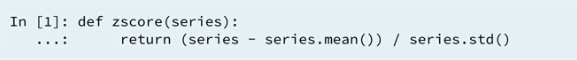
3.1 The Z-score

The z-score of a value is it's distance from the mean of it's population measured in units of standard deviation. This function is a transformation as it except a series as an input and return a conforming series

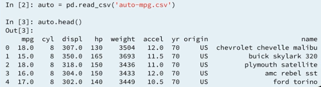
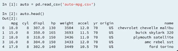
3.2 The automobile dataset

3.3 MPG z-score

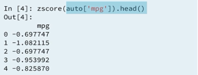
Looking at the second row, this means the mpg rating of 18.0 (may be 15.0, slip of toungh) for the 1970, buick skylark 320 is more than 1 standard deviation bellow the mean computed over all automobiles listed from 1970 to 1982.

3.4 MPG z-score

As an alternative we might want to normalize the mpg data independently by year, instead of over the whole population.

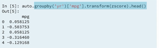
In this case normalized by year, the mpg rating for the buick skylark 320 is now only one half standard deviation bellow average amongs cars manufactured in 1970.

3.5 Apply transformation and aggregation

The .apply() method when used on a groupby object performs an arbitrary function on each of the groups. These functions can be aggregations, transformations or more complex workflows. The .apply() method will then combine the results in an intelligent way.

We know the agg method applies reduction and the transform method applies a function element wise to groups. In some cases, split a by combine operations do not needly for into aggregation or transformation for those cases we use apply. As an example:

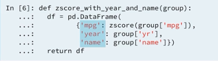
This new transformation is too complicated for transform so use apply instead. The output is the same z-score normalized mpg rating along with the name and year of manufacture for each automobile.

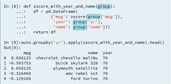
Lets take a look at the function zscore_with_year_and_name again. This functon is called 13 times once for each year between 1970 and 1982. That is once for each group. We didn't select any particular columns after grouping, so all of the columns retained in the sub groups used by the method apply. Within the function the output dataframe has three columns specified as dictionary keys. The dictionary values are selections from the input group. We transform the mpg column and take the original values from the year and name columns. After z-score with year and name has been called 13 times, the apply function recombined the outputs in a dataframe with 390 rows.

3.6 Example 3: Filling missing data (imputation) by group

Link

Many statistical and machine learning packages cannot determine the best action to take when missing data entries are encountered. Dealing with missing data is natural in pandas (both in using the default behavior and in defining a custom behavior). In Chapter 1, you practiced using the .dropna() method to drop missing values. Now, you will practice imputing missing values. You can use .groupby() and .transform() to fill missing data appropriately for each group.

Your job is to fill in missing 'age' values for passengers on the Titanic with the median age from their 'gender' and 'pclass'. To do this, you'll group by the 'sex' and 'pclass'columns and transform each group with a custom function to call .fillna() and impute the median value.

The DataFrame has been pre-loaded as titanic. Explore it in the IPython Shell by printing the output of titanic.tail(10). Notice in particular the NaNs in the 'age' column.

# Create a groupby object: by_sex_class
by_sex_class = titanic.groupby(['sex', 'pclass'])

# Write a function that imputes median
def impute_median(series):
    return series.fillna(series.median())

# Impute age and assign to titanic['age']
titanic.age = by_sex_class.age.transform(impute_median)

# Print the output of titanic.tail(10)
print(titanic.tail(10))

3.7 Example 4 : Other transformations with .apply

The .apply() method when used on a groupby object performs an arbitrary function on each of the groups. These functions can be aggregations, transformations or more complex workflows. The .apply() method will then combine the results in an intelligent way.

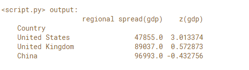
In this exercise, you're going to analyze economic disparity within regions of the world using the Gapminder data set for 2010. To do this you'll define a function to compute the aggregate spread of per capita GDP in each region and the individual country's z-score of the regional per capita GDP. You'll then select three countries - United States, Great Britain and China - to see a summary of the regional GDP and that country's z-score against the regional mean.

The 2010 Gapminder DataFrame is provided for you as gapminder_2010. Pandas has been imported as pd.

The following function has been defined for your use:

def disparity(gr):
    # Compute the spread of gr['gdp']: s
    s = gr['gdp'].max() - gr['gdp'].min()
    # Compute the z-score of gr['gdp'] as (gr['gdp']-gr['gdp'].mean())/gr['gdp'].std(): z
    z = (gr['gdp'] - gr['gdp'].mean())/gr['gdp'].std()
    # Return a DataFrame with the inputs {'z(gdp)':z, 'regional spread(gdp)':s}
    return pd.DataFrame({'z(gdp)':z , 'regional spread(gdp)':s})

# Group gapminder_2010 by 'region': regional
regional = gapminder_2010.groupby('region')

# Apply the disparity function on regional: reg_disp
reg_disp = regional.apply(disparity)

# Print the disparity of 'United States', 'United Kingdom', and 'China'
print(reg_disp.loc['United States','United Kingdom','China'](/upalr/Python-camp/wiki/'United-States','United-Kingdom','China'))

4 Groupby and filtering

4.1 The automobile dataset

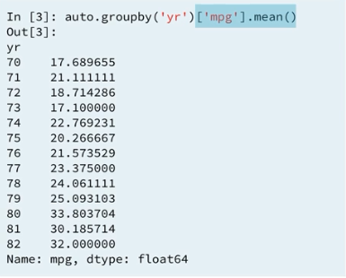
4.2 Mean MPG by year

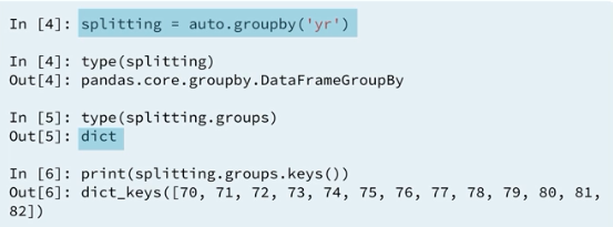
4.3 Groupby object

But what if we want the yearly average only for cars built by .To answer this question, we have to filter the groups before aggregating.

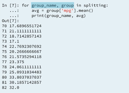
4.4 Groupby object : iteration

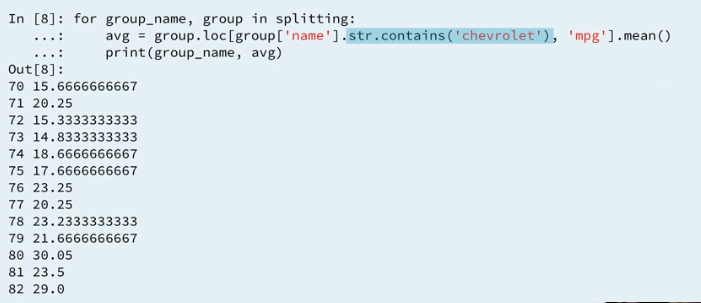
4.5 Groupby object : iteration and filtering

4.6 Groupby object : comprehension

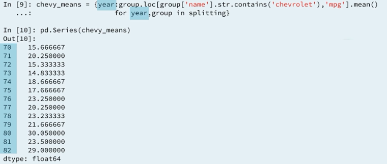
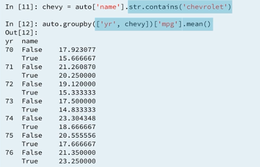
4.7 Boolean groupby

Seems like apply and filter a Dataframe ar column shoho pawa possible with exising index.

4.8 Ways of filtering

4.8.1 Example: Grouping and filtering with .apply()

Grouping and filtering with .apply()

By using .apply(), you can write functions that filter rows within groups. The .apply() method will handle the iteration over individual groups and then re-combine them back into a Series or DataFrame.

In this exercise you'll take the Titanic data set and analyze survival rates from the 'C' deck, which contained the most passengers. To do this you'll group the dataset by 'sex' and then use the .apply() method on a provided user defined function which calculates the mean survival rates on the 'C' deck:

def c_deck_survival(gr):

    c_passengers = gr['cabin'].str.startswith('C').fillna(False)

    return gr.loc[c_passengers, 'survived'].mean()

The DataFrame has been pre-loaded as titanic.

Instructions:

• Group titanic by 'sex'. Save the result as by_sex.
• Apply the provided c_deck_survival function on the by_sex DataFrame. Save the result as c_surv_by_sex.
• Print c_surv_by_sex.

# Create a groupby object using titanic over the 'sex' column: by_sex
by_sex = titanic.groupby('sex')

# Call by_sex.apply with the function c_deck_survival and print the result
c_surv_by_sex = by_sex.apply(c_deck_survival)

# Print the survival rates
print(c_surv_by_sex)

4.8.2 Example : Grouping and filtering with .filter()

Grouping and filtering with .filter()

You can use groupby with the .filter() method to remove whole groups of rows from a DataFrame based on a boolean condition.

In this exercise, you'll take the February sales data and remove entries from companies that purchased less than 35 Units in the whole month.

First, you'll identify how many units each company bought for verification. Next you'll use the .filter() method after grouping by 'Company' to remove all rows belonging to companies whose sum over the 'Units' column was less than 35. Finally, verify that the three companies whose total Units purchased were less than 35 have been filtered out from the DataFrame.

Instructions:

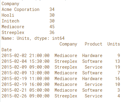
Group salesby'Company'. Save the result as by_company. Compute and print the sum of the 'Units'column ofby_company. Call .filter()onby_companywithlambda g:g['Units'].sum() > 35 as input and print the result.

# Read the CSV file into a DataFrame: sales
sales = pd.read_csv('sales.csv', index_col='Date', parse_dates=True)

# Group sales by 'Company': by_company
by_company = sales.groupby('Company')

# Compute the sum of the 'Units' of by_company: by_com_sum
by_com_sum = by_company['Units'].agg('sum')
print(by_com_sum)

# Filter 'Units' where the sum is > 35: by_com_filt
by_com_filt = by_company.filter(lambda g : g['Units'].sum() > 35)
print(by_com_filt)

Output:

4.8.3 Filtering and grouping with .map()

You have seen how to group by a column, or by multiple columns. Sometimes, you may instead want to group by a function/transformation of a column. The key here is that the Series is indexed the same way as the DataFrame. You can also mix and match column grouping with Series grouping.

In this exercise your job is to investigate survival rates of passengers on the Titanic by 'age' and 'pclass'. In particular, the goal is to find out what fraction of children under 10 survived in each 'pclass'. You'll do this by first creating a boolean array where True is passengers under 10 years old and False is passengers over 10. You'll use .map() to change these values to strings.

Finally, you'll group by the under 10 series and the 'pclass' column and aggregate the 'survived' column. The 'survived' column has the value 1 if the passenger survived and 0 otherwise. The mean of the 'survived' column is the fraction of passengers who lived.

The DataFrame has been pre-loaded for you as titanic.

Instrutions:

• Create a Boolean Series of titanic['age'] < 10 and call .map with {True:'under 10', False:'over 10'}.
• Group titanic by the under10 Series and then compute and print the mean of the 'survived' column.
• Group titanic by the under10 Series as well as the 'pclass' column and then compute and print the mean of the 'survived'

# Create the Boolean Series: under10
under10 = (titanic['age'] < 10).map({True:'under 10', False:'over 10'})

# Group by under10 and compute the survival rate
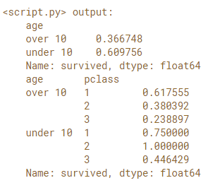
survived_mean_1 = titanic.groupby(under10)['survived'].agg('mean')
print(survived_mean_1)

# Group by under10 and pclass and compute the survival rate
survived_mean_2 = titanic.groupby([under10, 'pclass'])['survived'].agg('mean')
print(survived_mean_2)