Graduate Student Test: Weather Model CCN Experiment - ufs-community/ufs-weather-model GitHub Wiki
This test assesses how easy it is to access and run a UFS code, modify a configuration file to change a physics parameter, re-run the code and then compare results for the UFS Weather Model. It is an example of a code usability evaluation following the "Graduate Student Test" protocol developed for the Unified Forecast System (UFS). For more information about the feedback we've received, please visit the "Graduate Student Test" page.
There is a brief description of the model code in the UFS Weather Model User's Guide, and pointers to additional documentation.
In order to perform the test, you will run the model for 24 hours, make a change in the namelist to increase the concentration of cloud condensation nucleii (CCN), and perform another 24 hour run with this change. Then you will compare the total cloud cover field before and after the change.
Cloud condensation nuclei (CCN) are small particles suspended in the atmosphere on which water vapor condenses. The number of nuclei per cubic centimeter is used in the microphysics parameterization. With more CCN in the air, cloud water is distributed over a larger number of smaller drops. This hinders the development of precipitation processes, so droplets stay suspended and cloud coverage is higher. Even after just twenty four hours, an increase can be seen in the cloud cover field. As the forecast progresses, nonlinear processes take place and can change this simple interpretation.
Follow the instructions in Getting Started to run the C96 case for 24 hours (i.e. simple-test-case). The version of the physics used in this test is the GFSv15p2 package, which is the default. You will use the same tag specified on the Getting Started page.
Once your run is complete, move the run directory (i.e. simple-test-case) to simple-test-case.control. This folder will be used to compare the control run to the run with the modified concentration of CCN.
% cd <working_directory>
% mv simple-test-case simple-test-case.control
Follow the Download a Test Case instructions on the Getting Started page to once again untar the simple-test-case.tar.gz file.
Now edit the concentration of CCN in the input.nml namelist file.
% cd <working_directory>/simple-test-case
% <your_preferred_editor> input.nml
Change:
ccn_l = 300.
ccn_o = 100.
to:
ccn_l = 900.
ccn_o = 300.
Now rerun the test, once more following the Run the Test Case instructions on the Getting Started page.
Once your run is complete, move the run directory (i.e. simple-test-case) to simple-test-case.test. This folder will be used to compare the run with the the modified concentration of CCN to the control run.
% cd <working_directory>
% mv simple-test-case simple-test-case.test
Changing the concentration of CCN creates a noticeable difference in the total cloud cover. Now that you've completed both runs compare the total cloud cover before and after the CCN change.
A simple way to look at the difference is to use the combination of the NCDIFF differencing capability that is part of netCDF Operators (NCO) and Ncview.
To use NCDIFF + Ncview load the following modulefiles:
| System | Modules |
|---|---|
| Cheyenne | module load nco/4.7.9 ncview/2.1.7 |
| Stampede2 | module load nco/4.6.9 netcdf hdf5 udunits ncview/2.1.7 |
| Hera | module load intel nco ncview |
Differences can be computed using the netCDF Operator Tools:
% cd <working_directory>
% ncdiff simple-test-case.test/phyf024.nc simple-test-case.control/phyf024.nc phyf024_diff.nc
The resulting phyf024_diff.nc file can be visualized by Ncview:
% ncview phyf024_diff.nc
Note that if you receive the following error 'display: unable to open X server' then you must log out and log in with -X as an argument passed into ssh. The -X argument enables X11 forwarding.
Your Ncview output of Atmospheric Column Total Cloud Cover Difference (tcdc_aveclm) after changing the range to -35:35 should look like this.
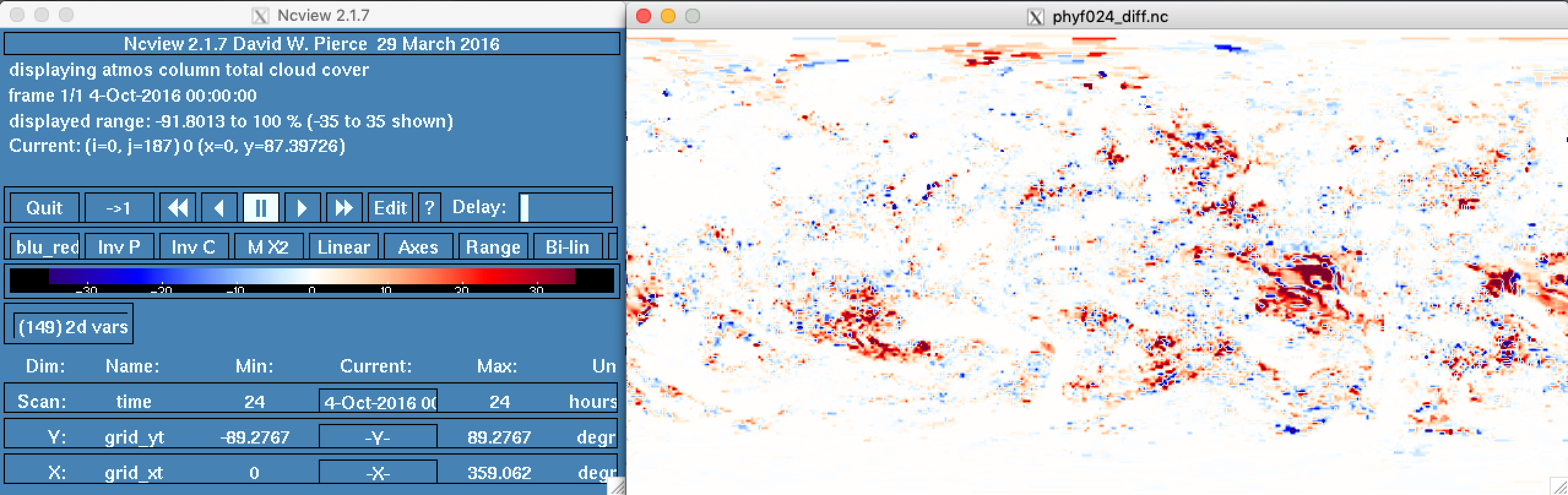 |
Another option for looking at the difference is to use NCL with the following script. By default, this script plots the differences between control and test runs for 2m Temperature (tmp2m), Total Precipitation (tprcp), and Atmospheric Column Total Cloud Cover (tcdc_aveclm) at 24h.
You can download the script here:
https://raw.githubusercontent.com/wiki/ufs-community/ufs-weather-model/tools/plot_ufs_phyf_diff.ncl
To run this NCL script execute the following commands. This script will produce png files for each variable being plotted.
% cd <working_directory>
% wget https://raw.githubusercontent.com/wiki/ufs-community/ufs-weather-model/tools/plot_ufs_phyf_diff.ncl
% ncl plot_ufs_phyf_diff.ncl 'c="simple-test-case.control"' 't="simple-test-case.test"'
Your NCL output of Atmospheric Column Total Cloud Cover Difference (tcdc_aveclm) should look like this:
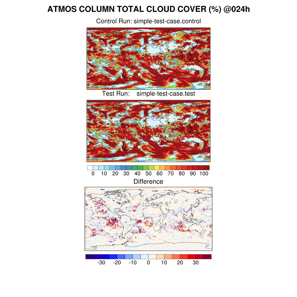 |