ERPLAB Studio: Average Across ERPsets - ucdavis/erplab GitHub Wiki
The Average Across ERPsets (Grand Average) panel is used to average together the ERPsets that are selected in the ERPsets panel. That is, the average across the selected ERPsets is computed for each bin. The most common use for this is to create a grand average across subjects. It can also be used to average across ERPsets for a single participant (e.g., ERPsets for different sessions). This routine can be used only if all of the ERPsets being averaged together contain the same number of bins, channels, and sample points.
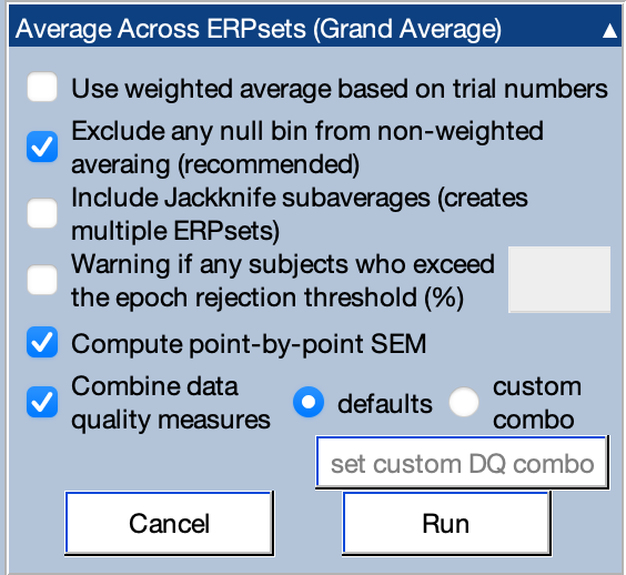
Ordinarily, each ERPset being averaged together receives equally weighting in the average that is created by this routine. That is, the ERP waveforms in the separate ERPsets are simply summed together and then divided by the number of ERPsets. However, there is an option for averaging in a manner that is weighted by the number of trials that contributed to each average (a "weighted average"). Imagine, for example, that you were averaging together two sessions from a given subject, with each session stored in a separate ERPset, and bin 1 contained 10 trials in the first session and 90 trials in the second session. If you enable weighted averaging, the average of bin 1 would be calculated as 10 times the waveform from session one plus 90 times the waveform from session two, and then divided by the total number of trials (10+90). This gives each trial equal weight in the final average.
If one of the bins in one of the ERPsets did not actually have any trials (e.g., due to artifacts), this bin will have no weight and will not impact the grand average if you are computing weighted averages. However, this can really mess up the default unweighted averaging procedure, because that bin will be flatlined for that ERPset (i.e., the voltage will be zero at all time points). These "null bins" can be automatically excluded if you select the option labeled Excludes any null bin from non-weighted averaging. Keep in mind, however, that the presence of a null bin often means that there is a problem somewhere in your data analysis pipeline that needs to be fixed. For example, conventional statistics cannot be used if you have no data in one condition in one of your subjects. Also, using this option will mean that different subjects contribute to the different bins in the grand average. Thus, you should use this option carefully.
There is also an option for having the routine warn you about subjects who have an excessive number of rejected trials. For example, you might want to exclude any subjects for whom over 25% of trials were rejected (see Chapter 6 in An Introduction to the Event-Related Potential Technique). This option provides a convenient way of checking this (but it does not automatically exclude the subjects).
This tool can make leave-one-out grand averages for use with the Jackknife statistical technique (see Chapter 10 in An Introduction to the Event-Related Potential Technique). When you select this option with N ERPsets selected, the routine will create N+1 grand averages. The first one (named with an “-0” extension) is the ordinary grand average. Each additional grand average will exclude 1 of the N ERPsets. For example, the grand average ERPset named with a “-1” extension will be the average of all ERPsets except the first one, and the grand average ERPset named with a “-2” extension will be the average of all ERPsets except the second one.
There is an option for calculating the point-by-point standard error (SEM) of the mean across the ERPsets. This provides the SEM across ERPsets at each time point. In other words, for each ERPset, we find the voltage at a given time point for a given bin and channel, and we compute the SEM [SD ÷ sqrt(number of ERPsets)]. If the point-by-point SEM across trials was computed at the [time of averaging, that information is discarded and replaced with this new SEM information. Whereas the point-by-point SEM across trials that can be calculated at the time of averaging reflects the data quality at that time point, the point-by-point SEM across ERPsets calculated here reflects both the data quality and true differences among ERPsets (e.g., true differences in amplitude across participants that would be present even with an infinite number of trials).
If data quality metrics such as the standardized measurement error were computed when the ERPsets were created (e.g., at the time of averaging), it is possible to compute aggregate measures of data quality across the ERPsets when the grand average of the waveforms is computed by checking Compute data quality measures. By default, these measures will be computed as the root mean square (RMS) across whatever data quality measures exist in the ERPsets. Note that the data quality measures can be combined only if the same measures exist in all ERPsets being combined.
The process of aggregating values across ERPsets can be customized by selecting custom combo and clicking the Set custom DQ combo button, which brings up the window shown in the screenshot below. This window shows the existing data quality measures in the input ERPsets (upper left) and lists the methods than can be used to combine them for the output ERPset (upper right). You simply select a measure and a combination method and then click the Add this button.
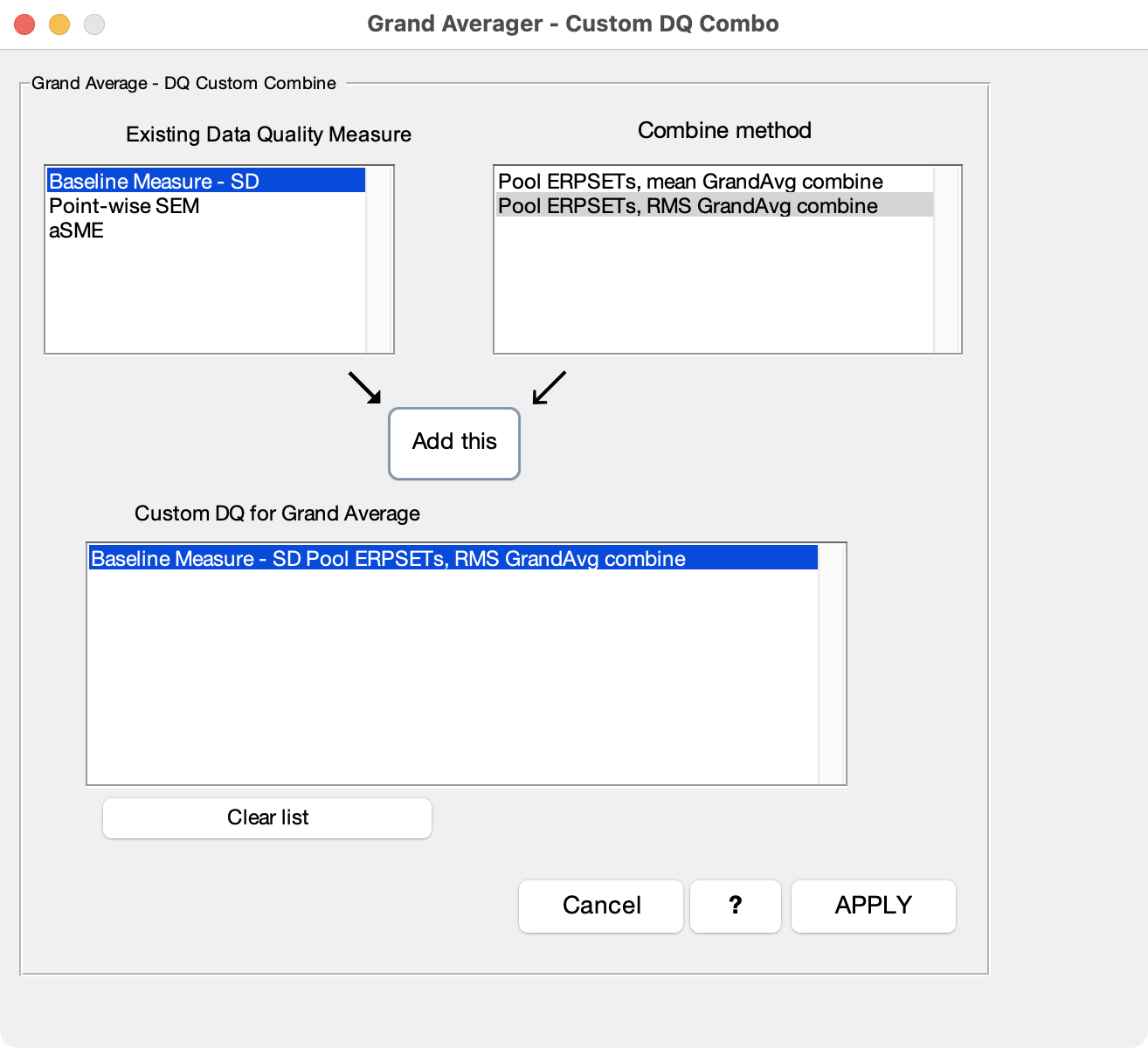
The simplest way to combine data quality metrics is to simply take the mean of the values across the input ERPsets (Pool ERPSETs: mean GrandAvg combine). In many cases, however, it is better to combine them by taking the Root Mean Square (RMS) of the values (Pool ERPSETs: RMS GrandAvg combine). Using RMS rather than the mean gives you a better idea of how the single-participant data quality will impact the variability in your amplitude or latency measurements across participants, your effect sizes, and your statistical power (see our original paper describing the standardized measurement error).