ERP Bin Operations - ucdavis/erplab GitHub Wiki
The Bin Operations tool allows you to compute new bins that are combinations of the bins in the current ERP structure. For example, you can average multiple bins together, and you can compute difference waves. To use it, you will write simple equations that describe how the new bin is computed. For example, to create a new Bin 3 that is the average of the current Bin 1 and Bin 2, you would write the following equation: b3 = (b1+b2)/2 (or b3 = 0.5b1 + 0.5b2). You will usually want to create a label for a new bin by putting something like label Average of Bins 2 and 3 at the end of the equation.
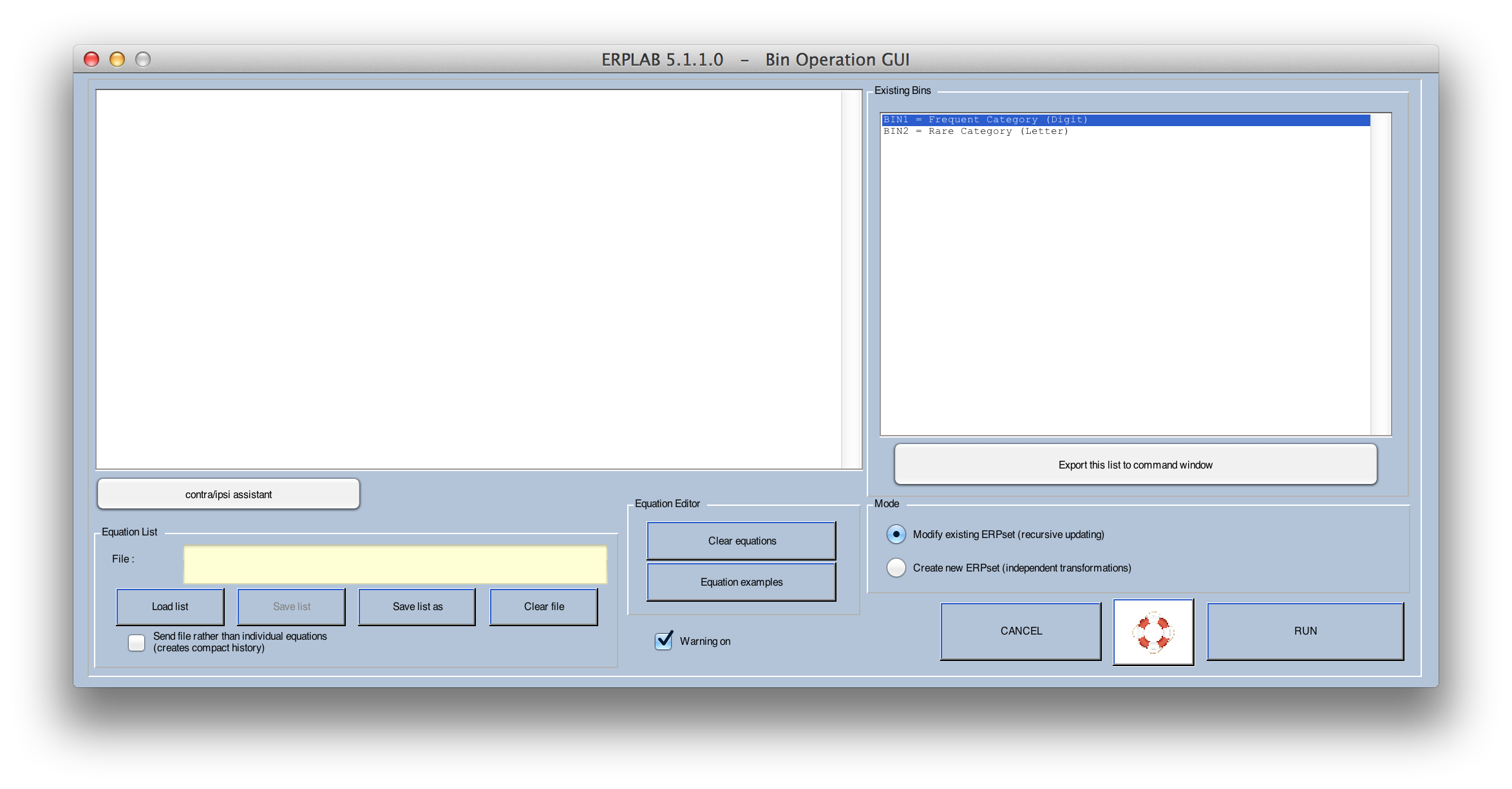
In ERPLAB Classic, this tool is accessed by selecting ERPLAB > ERP Operations > ERP Bin Operations.
In ERPLAB Studio, this tool is accessed from the Bin Operations panel in the ERP tab. In ERPLAB Studio, some of the options are accessed using the Advanced button.
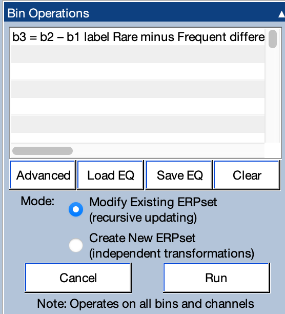
In the examples shown above, a rare-minus-frequent difference wave is being created from an oddball paradigm using the equation b3 = b2 – b1 label Rare minus Frequent difference wave. You can create multiple bins by providing multiple equations, one on each line. You just type the equations into the text box in the GUI.
You can save the equations in a text file and load them again later. This is accomplished in ERPLAB Studio with the SaveEQ and LoadEQ buttons, and it is accomplished in ERPLAB Classic using Save list, Save list as, and Load list.
Note for scripting: Ordinarily, the equations are sent to the Matlab function as a set of strings (a cell array). With a long list of equations, this will lead to a very complicated function call in your history. If you select the option for Send file rather than individual equations, the file will be sent instead of the equations, making the history simpler (which is convenient if you plan to turn the history into a script). But the same bin operations will be performed either way.
You can use bin# or b# to specify a bin, and virtually any standard mathematical equation can be used. Here are some examples:
- B5 = ((b1+b2)/2) – ((b3+b4)/2) label Average of bins 1 and 2 minus average of bins 3 and 4
- Bin5 = sqrt(b2^2 + b3^2) label Square root of sum of squared bins 2 and 3
- b5 = abs(b4) label Absolute value of bin 4 (rectification)
- bin5 = b4 + 1 label Add an offset of 1 microvolt to the entire bin 4 waveform
In addition, you can use a function named wavgbin (for "weighted average bin") to averages together a set of bins, weighted by the number of epochs that contributed to each bin. For example, if bin 1 was created by averaging together 10 epochs, and bin 2 was created by averaging together 90 epochs, you could create a bin that is equivalent to what you would have gotten by averaging these 100 epochs together during the initial averaging process (which is the same as "(10bin1 + 90bin2)/100"). It is used as follows:
- Bin3 = wavgbin(1, 2) label Weighted average of bins 1 and 2
- Bin9 = wavgbin(1:8) label Weighted average of bins 1 through 8
- Bin20 = wavgbin(1:4,6,9,12:15) label Weighted average of bins 1-4, 6, 9, and 12-15
Modes of Operation
Bin Operations has two modes of operation. In Modify Existing ERPset mode, the equations modify existing bins and/or add new bins within the current ERPset. This mode is great for simple operations, like adding a new bin containing a difference wave or the average of other bins. However, it can lead to unexpected results if you are modifying an existing bin (because it operates "recursively"). Also, although you can add new bins with this mode, you cannot delete bins.
When you use this mode, the bin on the left side of each equation should be listed as "b1 =" or "bin1 =" (as in the examples given above).
In Create New ERPset mode, the current ERPset serves as the input to equations, and a new set of bins is created in a new ERPset. This mode requires you to provide equations for all the bins you are creating, even if some of them are simply copies of the input bins. This mode is particularly useful for creating a new ERPset that does not contain the original bins. For example, you could use it to create a new ERPset that has a set of difference waves but no longer contains the original "parent" waves.
When you are creating a new ERPset, each bin equation must begin with with "nb " or "newbin =" as a reminder that you are creating a new bin within a new ERPset. For example, if the input ERPset had bins 1 and 2, and you want to create a new ERPset with just a single bin containing the difference between the original bins 1 and 2, you would use an equation like:
- nb1 = bin2 - bin1 label Difference Wave
Order of Bins
Bins must always be defined in ascending order, starting with Bin 1. For example, if you are creating a new ERPset, your first equation will begin with newbin1 =, your second equation will begin with newbin2 =, and so on.
When you are modifying an existing ERPset, your list of equations does not need to re-define the existing bins. However, any new bins that are defined must occur in ascending order, and the result cannot have any missing bins. For example, if the current ERPset contains bins 1-10, you could have a list of equations like this:
- B3 = B1 – B2 label Re-definition of bin 3
- B11 = B3 – B5 label Create new bin 11 as difference between bin 5 and newly updated bin 3
- B12 = B11^2 label Create new bin 12 that is the new bin 11 squared
However, you could not have a list of equations that began with bin 12 (because bin 11 has not yet been defined) or a list in which bin 12 came before bin 11.
Specifying subsets of channels (especially to compute contra versus ipsi)
You can specify different subsets of channels for the different bins being used in a given equation, which is especially useful for isolating the N2pc and LRP components. For example, if you are trying to compute a lateralized readiness potential (LRP) waveform, you will want to subtract trials with an ipsilateral response from trials with a contralateral response, averaged across the left and right hemispheres. That is, you want to make a contralateral average (left-hemisphere electrode sites for right-hand responses averaged with right-hemisphere electrode sites for left-hand responses) and an ipsilateral average (left-hemisphere sites for left-hand responses averaged with right-hemisphere sites for right-hand response) and compute the difference. This section will describe how to do this manually. The next section will describe the contra/ipsi assistant, which can do much of the work for you.
To do this manuall, you first provide equations that define sets of electrodes corresponding to the left and right hemispheres. Imagine that the electrode sites 1-6 are as follows 1=F3, 2=F4, 3=C3, 4=C4, 5=P3, 6=P4. And imagine that Bin 1 corresponds to left-hand responses whereas Bin 2 corresponds to right-hand responses. The following shows how you would define left- and right-hemisphere groups and use them to form a contralateral waveform (new Bin 1), an ipsilateral waveform (new Bin 2), and a contra-minus-ipsi difference wave (new Bin 3):
- LH = [1 3 5]
- RH = [2 4 6]
- b1 = (b2@LH + b1@RH)/2 label Average Contra
- b2 = (b1@LH + b2@RH/2 label Average Ipsi
- b3 = ((b2@LH + b1@RH)/2) – ((b1@LH + b2@RH)/2) label Average Contra Minus Ipsi
In this example, we first define two electrode groups, named LH and RH (containing the left-hemisphere and right-hemisphere electrode sites, respectively). We then specify which electrode groups should be used for each bin by connecting the bin number and the electrode group with @ symbol.
The resulting ERPset would have only 3 channels (automatically labeled 'F3/4' 'C3/4' 'P3/4'). Because the new bins have fewer channels than the old bins, you would not be able to update the existing ERPset when creating these new bins, so you would need to use Create New ERPset mode.
You can have ERPLAB automatically create left- and right-hemisphere groups on the basis of the channel labels. Specifically, the "LH =" and "RH =" lines in the above example could be replaced by the following line:
- [LH RH] = splitbrain(ERP)
The splitbrain() function finds pairs of electrodes whose names are identical except for ending with consecutive odd (for left-hemisphere) and even (for right-hemisphere) numbers (following the International 10/20 System convention). For example, it would treat Fp1 and Fp2 as corresponding left-right pairs. But the electrode names do not have to be standard 10/20 names (e.g., it would treat Temporal125 and Temporal126 as corresponding left-right pairs). Any electrode sites that don't end in a number will be excluded from the channel groups (e.g., Fz), and will generate a warning (which you can usually ignore because you usually want to exclude such electrodes when creating left-right pairs).
Note that, although "LH" and "RH" were used to name the electrode groups in these examples, you can use any strings to name the groups. Also, this can be used to create any kind of channel subsets that you'd like, not just left hemisphere and right hemisphere subsets.
Using the Contra/Ipsi Assistant
The GUI contains a button labeled contra/ipsi assistant (accessed from the Advanced button in ERPLAB Studio). This button brings up the GUI shown below, which will create the equations for making the contra and ipsi waveforms (for most experiments).
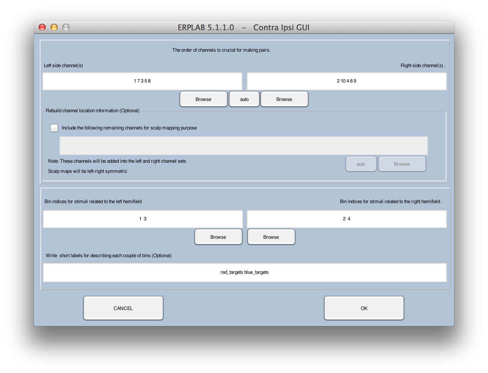
The first two text boxes are used to list the left- and right-hemisphere channel pairs. You need to make sure that the channels are in the same order for both the left and right sides (e.g., channels F3, C3, and P3 [in that order] for the left side and F4, C4, and P4 [in that order] for the right side). If you click the auto button, ERPLAB will attempt to find the appropriate channels for you (on the basis of standard naming conventions).
You then need to specify which bins correspond to trials on which attention will be directed to the left versus right hemifields. For example, imagine that you have the following bins:
- Bin 1: Red target in the left visual field
- Bin 2: Red target in the right visual field
- Bin 3: Blue target in the left visual field
- Bin 4: Blue target in the right visual field
Bins 1 and 3 would go into the left hemifield text box, and bins 2 and 4 would go into the right hemifield text box.
Bins 1 and 2 will then be converted into a contra bin and an ipsi bin for the red targets, and Bins 3 and 4 will then be converted into a contra bin and an ipso bin for the blue targets. You would provide labels for these new bins (e.g., label red_targets for the new bins 1 and 2, and label blue_targets for the new bins 3 and 4).
Once you click OK, you will get a set of equations like this:
- Lch = [ 1 7 3 5 8]
- Rch = [ 2 10 4 6 9]
- nbin1 = 0.5bin1@Rch + 0.5bin2@Lch label red_targets Contra
- nbin2 = 0.5bin1@Lch + 0.5bin2@Rch label red_targets Ipsi
- nbin3 = 0.5bin3@Rch + 0.5bin4@Lch label blue_targets Contra
- nbin4 = 0.5bin3@Lch + 0.5bin4@Rch label blue_targets Ipsi
To create contra-minus-ipsi waveforms from the bins in the new ERPset, you would run BINLISTER a second time with the equations shown below (using the Modify Existing ERPset mode):
- bin5 = bin1 - bin2 label red_targets Contra-Ipsi
- bin6 = bin3 - bin4 label blue_targets Contra-Ipsi