Introduction to QTL Analysis - ua-datalab/Bioinformatics GitHub Wiki

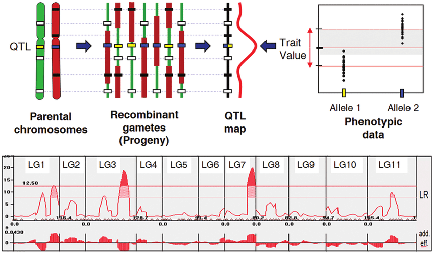
Figure from Genomics, Domestication, and Evolution of Forest Trees, Sederoff et al., 2010

---

---

---

---

QTL (Quantitative Trait Locus) mapping is the process of identifying genomic regions associated with variation in quantitative traits. Unlike single-gene traits, quantitative traits (e.g., height, yield, disease resistance) are controlled by multiple genes and environmental factors. QTL mapping uses genetic markers to locate these regions.

Quantitative trait mapping is used in biomedical, agricultural, and evolutionary studies to find causal genes for quantitative traits, to aid crop and breed selection in agriculture, and to shed light on natural selection. Examples of quantitative traits include cholesterol level, plant yield, or egg size, all of which are continuous variables.

The goal of quantitative trait locus (QTL) analysis is to identify genomic regions linked to a phenotype, to map these regions precisely, and to define the effects, number, and interactions of QTL.

QTL analysis in experimental crosses requires two or more strains that differ genetically with regard to a phenotype of interest. Genetic markers, such as SNPs (Single Nucleotide Polymorphisms) or microsatellites, distinguish between parental strains in the experimental cross.

Markers that are genetically linked to a phenotype will segregate more often with phenotype values (high or low values, for example), while unlinked markers will not be significantly associated with the phenotype. The markers themselves might be associated with the phenotype but are not causal. Rather, markers may be associated with the phenotype through linkage to nearby QTL. They serve as signposts indicating the neighborhood of a QTL that influences a phenotype . Covariates such as sex or diet can also influence the phenotype.

It is extremely difficult to cover QTLs in a single hour; In today's workshop we are going to cover:

• Study design, experimental crosses and "what does a pipeline look like"?
• QTL mapping methods

---

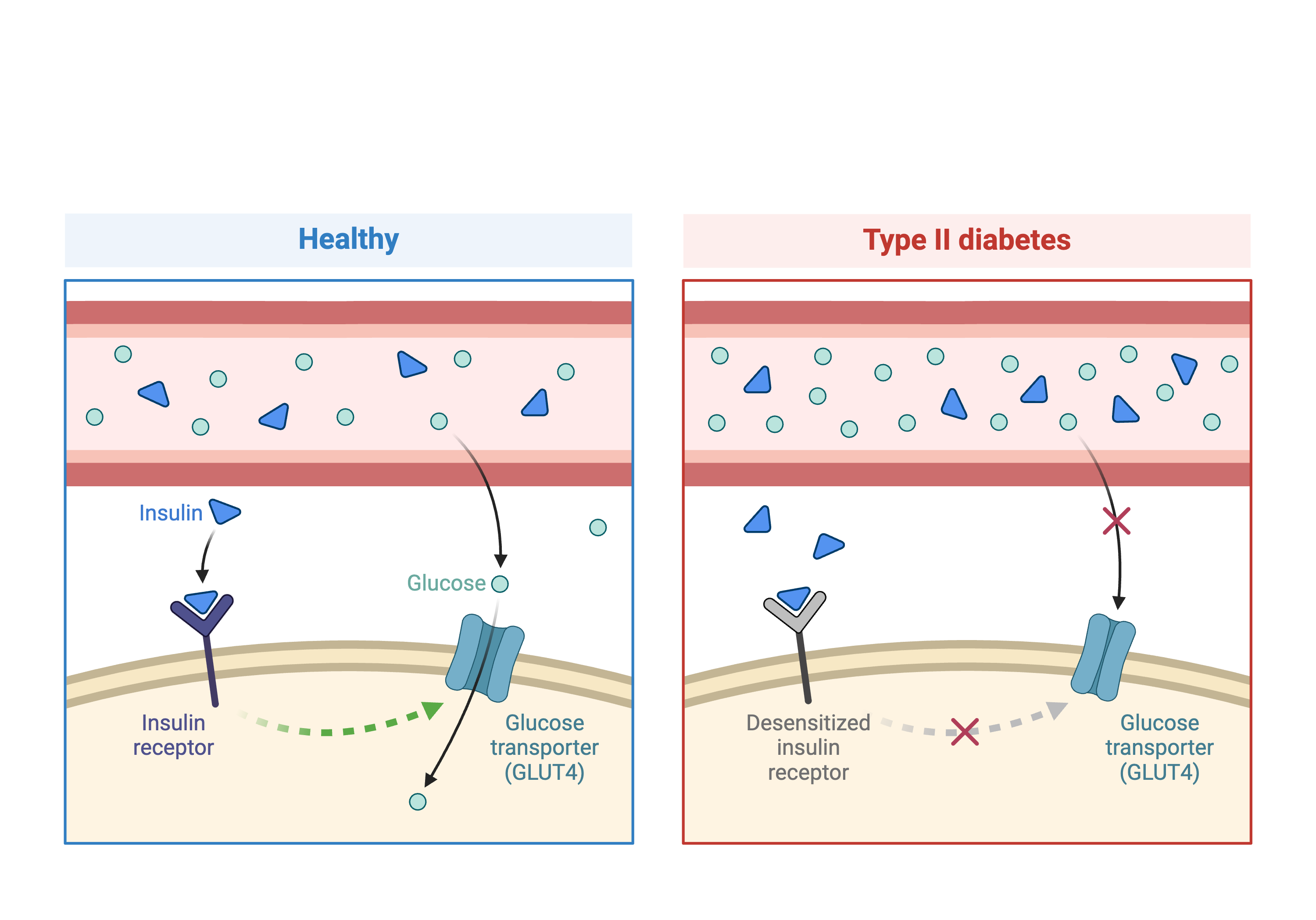
In this workshop we will be analyzing data from a mouse experiment involving Type 2 diabetes (T2D). There are two types of diabetes: type 1, in which the immune system attacks insulin-secreting cells and prevents insulin production, and type 2, in which the pancreas makes less insulin and the body becomes less responsive to insulin.

This study is from Tian et al. and involves an intercross between the diabetes-resistant C57BL/6J (B6 or B) strain and the diabetes-susceptible BTBR T+ tf/J (BTBR or R) strain mice carrying a Leptin^ob/ob mutation.

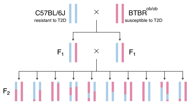
The mutation prevents the production of leptin, a hormone that regulates hunger and satiety. When leptin levels are low (or missing), the body does not receive satiety signals and continues to feel hunger. Leptin^ob/ob mice continue to eat and become obese. Obesity is one of the risk factors for T2D and this experiment sought to use genetic variation between B6 and BTBR strains to identify genes which influence T2D.

The experiment analyzes circulating insulin levels and pancreatic islet gene expression, mapping circulating insulin levels to identify genomic loci which influence insulin levels. SNPs that differ between C57BL/6J and BTBR and pancreatic islet gene expression data are used to identify candidate genes.

QTL mapping data consists of a set of tables of data: sample genotypes, phenotypes, marker maps, etc. These different tables are in different comma-separated value (CSV) files. In each file, the first column is a set of IDs for the rows, and the first row is a set of IDs for the columns. For example, the genotype data file will have individual IDs in the first column, marker names for the rest of the column headers.

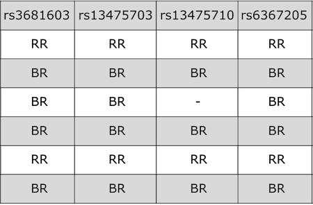
The sample genotype file above shows two alleles: B and R. These represent the founder strains for an intercross, which are C57BL/6 (BB) and BTBR (RR). The B and R alleles themselves represent the haplotypes inherited from the parental strains C57BL/6 and BTBR.

For the purposes of learning QTL mapping, this lesson begins with an intercross that has only 3 possible genotypes.

In QTL experiments, one needs to maps: a genetic marker map, and a physical map (if available).

An example of a genetic marker map looks like the following:

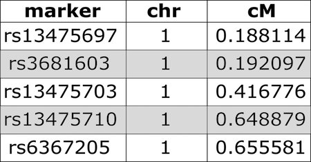
cM =centiMorgans, a unit for measuring genetic linkage. It is defined as the distance between chromosome positions (i.e., loci or markers) for which the expected average number of intervening chromosomal crossovers in a single generation is 0.01, often used to infer distance along a chromosome.

Whilst an example of a physical map looks like this:

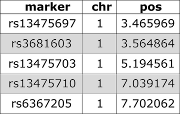
Note that location is provided in bases instead of centiMorgans.

Numeric phenotypes are separate from the often non-numeric covariates.

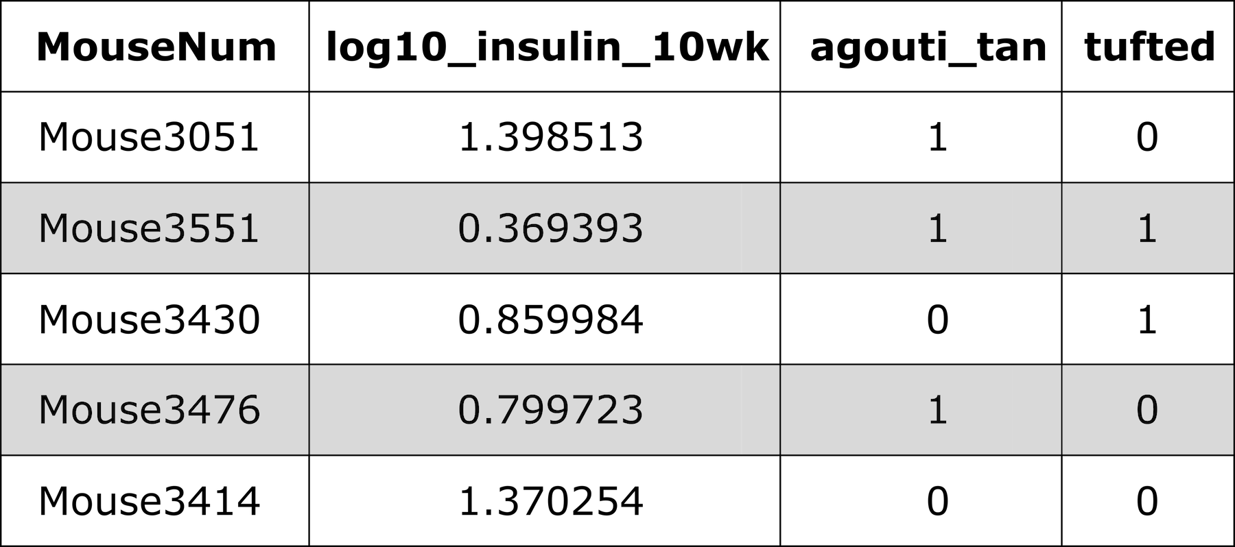
Agouti is a type of tan in mice (and other mammals), and tuf is how the fur is presented.

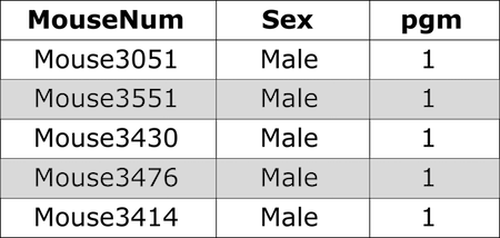
For gene expression data, we would have columns representing chromosome and physical position of genes, as well as gene IDs. The covariates shown below include sex and parental grandmother (pgm).

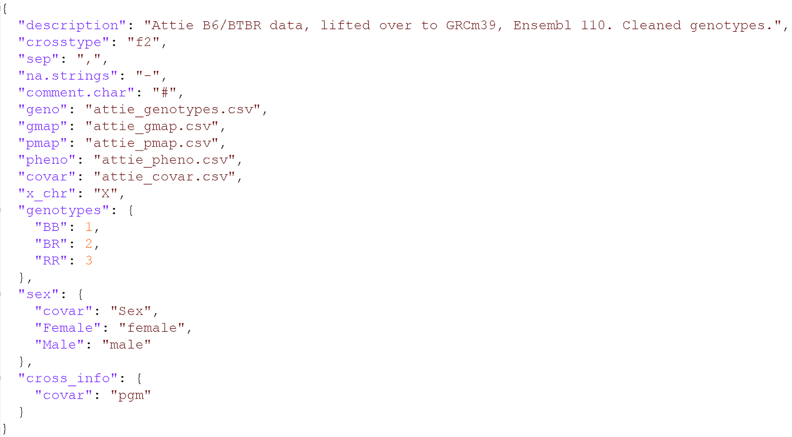
When working in R, the tool R/qtl2 requires an input YAML or JSON file that points out the various input csv files as well as other data:

Generally speaking, the full experiment looks like the following:

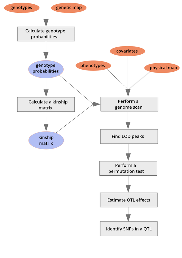
Here is a breakdown to the purpose and output of every step:

1. Calculate Genotype Probabilities
   • What it does: Uses marker data and recombination frequencies to estimate the probability of each individual having a specific genotype at unobserved locations in the genome.
   • Why it matters: Since genetic markers are not placed at every single base pair, this step fills in gaps to improve QTL detection accuracy.
2. Calculate a Kinship Matrix
   • What it does: Estimates the genetic relatedness between individuals based on shared alleles.
   • Why it matters: Correcting for kinship helps control for population structure effects, preventing false associations between markers and traits.
3. Perform a Genome Scan
   • What it does: Tests for statistical associations between genetic markers and the trait of interest across the entire genome.
   • Why it matters: Helps identify potential regions (QTLs) linked to trait variation.
4. Find LOD Peaks
   • What it does: Identifies locations in the genome where the Logarithm of the Odds (LOD) score is high, indicating strong evidence for a QTL.
   • Why it matters: Higher LOD scores suggest that a QTL is likely present in that genomic region.
5. Perform a Permutation Test
   • What it does: Randomly shuffles trait values among individuals multiple times to determine a threshold LOD score for statistical significance.
   • Why it matters: Ensures that detected QTLs are not just due to random chance.
6. Estimate QTL Effects
   • What it does: Quantifies how much each identified QTL contributes to variation in the trait.
   • Why it matters: Helps determine whether a QTL has a major or minor influence on the trait.
7. Identify SNPs in a QTL
   • What it does: Pinpoints specific single nucleotide polymorphisms (SNPs) within the QTL region that may be causal.
   • Why it matters: Identifying SNPs allows for further functional studies, gene discovery, and marker-assisted selection in breeding programs.

Due to time constraints we will not be able to follow every step of the pipeline. Rather, we will be looking at calculating genotype probabilities (and performing a genome scan with linear mix models), finding LOD peaks and identifying SNPs in a QTL.

We are going to be using the Carpentries-like lesson to simplify readability. Please follow the links below:

• Calculate Genotype Probabilites
  • Performing a Genome Scan with Linear Mix Models
• Using Permutations to Determine Significance Thresholds
  • Finding LOD Peaks
• Identify SNPs in a QTL

Following are notes for each of the steps above (without the code).

---

Purpose of Genotype Probabilities

• Genetic markers are not present at every base in the genome, so we infer missing genotypes using known marker data.
• This helps in QTL mapping by filling in gaps between observed markers.

Key Steps in Genotype Probability Calculation

• Uses recombination frequencies to estimate genotype probabilities at unobserved locations.
• Requires a genetic map (marker positions and recombination rates).
• Accounts for cross type (e.g., F2, backcross), as different breeding designs affect recombination patterns.

Why Genotype Probabilities Matter

• More accurate QTL detection by refining genotype estimates between markers.
• Helps in linkage mapping by considering how alleles segregate in a population.
• Reduces errors due to missing or sparse marker data.

Considerations

• High marker density improves genotype probability estimates.
• Recombination frequency calculations are critical for accuracy.
• Genotype probabilities are later used in QTL scans to detect trait-marker associations.

Purpose of a Linear Mixed Model (LMM) in Genome Scans

• Accounts for population structure and relatedness in QTL mapping.
• Helps reduce false positives by correcting for genetic background effects.

Key Concepts in LMM for QTL Mapping

• Fixed effects: The genetic marker being tested for association with the trait.
• Random effects: The genetic background (e.g., kinship or relatedness matrix) to control population structure.
• Uses a kinship matrix to model relatedness between individuals, preventing spurious associations.

Why Use LMM in Genome Scans?

• In structured populations (e.g., inbred lines, related individuals), ignoring relatedness can lead to incorrect QTL detection.
• LMM improves statistical power by distinguishing real QTL signals from background noise.
• Required when working with datasets where individuals aren’t fully independent (e.g., family-based studies).

Considerations

• Requires kinship matrix calculation before running the scan.
• More computationally intensive than simple genome scans.
• Used in both quantitative traits and binary trait mapping.

---

Purpose of a Permutation Test in QTL Mapping

• Determines the statistical significance of detected QTLs.
• Prevents false positives by setting a threshold for LOD scores based on randomization.

Key Concepts in Permutation Testing

• Trait values are shuffled randomly among individuals while keeping genotypes unchanged.
• The genome scan is repeated multiple times (e.g., 1,000 permutations).
• LOD scores from randomized data are compared to the real data to establish a threshold for significance.

Why Permutation Testing Matters

• Adjusts for multiple testing (since genome scans test thousands of markers).
• Ensures that only strong QTL signals are considered significant.
• Common practice in QTL studies to validate findings.

Considerations

• More permutations = more reliable threshold, but also higher computation time.
• The p-value of a QTL is estimated based on how often a random permutation produces an equal or higher LOD score.
• Different significance levels (e.g., 5%, 1%) can be used depending on study design.

Purpose of Finding LOD Peaks

• Identifies genomic regions (QTLs) significantly associated with a trait.
• Uses LOD (Logarithm of the Odds) scores to measure the strength of the association.

Key Concepts in Finding QTL Peaks

• LOD Score Calculation: Compares the likelihood of a QTL being present vs. absent at a given position.
• Threshold for Significance: Determined using permutation tests to avoid false positives.
• Peak Detection: The highest LOD scores indicate potential QTL locations.

Why Identifying LOD Peaks Matters

• Helps pinpoint candidate regions in the genome for further study.
• Peaks above the significance threshold indicate true QTLs rather than random associations.
• Understanding peak width and height gives insights into effect size and confidence intervals.

Considerations

• Higher LOD scores suggest stronger evidence for a QTL.
• Multiple peaks may indicate multiple QTLs influencing the trait.
• Fine-mapping and additional validation are needed to confirm candidate genes.

---

Purpose of Integrating Gene Expression Data in QTL Mapping

• Links genetic variants (QTLs) to gene expression changes.
• Helps identify expression QTLs (eQTLs), which influence gene activity.

Key Concepts in Gene Expression Integration

• Expression QTLs (eQTLs): QTLs that regulate gene expression rather than directly affecting a physical trait.
• Local vs. Distant eQTLs:
  • Cis-eQTLs: Near the gene they regulate.
  • Trans-eQTLs: Affect genes far from the QTL location.
• Statistical Association: Tests whether a genetic variant correlates with changes in gene expression levels.

Why Integrating Gene Expression Matters

• Connects genetic variation to molecular mechanisms behind traits.
• Helps distinguish causal genes from nearby variants.
• Can reveal gene regulatory networks influencing complex traits.

Considerations

• Requires both genotype and RNA expression data from the same individuals.
• Cis-eQTLs are easier to interpret than trans-eQTLs.
• Additional functional validation (e.g., CRISPR, RNA-seq) may be needed to confirm gene regulatory effects.