Introduction to GWAS - ua-datalab/Bioinformatics GitHub Wiki

📓 Notebook link: gwas.ipynb (raw)

Figure from Genomics, Domestication, and Evolution of Forest Trees, Sederoff et al., 2010

---

---

---

---

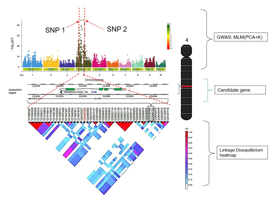
From: Genome-wide Association Study (GWAS) in TASSEL (GUI), from https://avikarn.com/2019-07-22-GWAS/ (honestly, a pretty good GUI friendly tutorial!)

Genome-Wide Association Studies (GWAS) are a method used in genetics to identify genetic variants associated with specific traits or diseases. The aim of GWAS is to identify single nucleotide polymorphisms (SNPs) of which the allele frequencies vary systematically as a function of phenotypic trait values (e.g., between cases with schizophrenia and healthy controls, or between individuals with high vs. low scores on neuroticism). Identification of trait-associated SNPs may subsequently reveal new insights into the biological mechanisms underlying these phenotypes.

The study requires a large number of data:

DNA Collection – DNA samples from (at least) two groups of people (or other organisms, to stay on topic we are going to be using humans as our species of interest):

• One group with the trait/disease (cases)
• One group without the trait/disease (controls)

Genotyping – each collected DNA needs to be genotyped in order to find single nucleotide polymorphisms (SNPs) across the population.

Each SNP is tested to see if it appears more frequently in cases than in controls. If a SNP is significantly more common in cases, it may be associated with the trait/disease.

There are obvious limitations to GWAS:

• GWAS finds associations, not direct causation
• Some traits are influenced by many genes and environmental factors
• Rare genetic variants may be missed
• Population bias
• Missing Heritability

These are important points to keep in mind when designing a GWA experiment.

Quantitative Trait Locus (QTL) analysis, which we have seen last week, is another approach used to study the genetic basis of traits, particularly in model organisms (e.g., plants, mice). Unlike GWAS, which scans genomes in large populations, QTL analysis is often performed in controlled crosses of genetically distinct parents.

Feature	GWAS	QTL Analysis
Study Type	Observational (in natural populations)	Experimental (crossing of selected individuals)
Resolution	High (identifies SNPs)	Lower (identifies larger chromosomal regions)
Trait Type	Common, complex traits	Quantitative traits in controlled settings
Data Source	Natural human populations	Laboratory or agricultural species
Population	Large, unrelated individuals	Genetically controlled crosses
Limitations	Detects associations but not causation, small effect sizes, missing heritability	Lower resolution, requires controlled breeding

GWAS and QTL analysis can go hand in hand: GWAS is best for studying complex traits in large populations, whilst QTL is best for controlled studies and finding major-effect genes.

1. QTL mapping can validate GWAS findings:
   • GWAS identifies SNPs associated with a trait in natural populations, but these associations are often weak and require further validation.
   • QTL analysis, which uses controlled crosses, can help confirm whether a genomic region linked to a GWAS-identified SNP truly influences the trait.
   • Example: In Arabidopsis thaliana, a GWAS might find an SNP linked to drought tolerance. A QTL study in controlled crosses can determine if this SNP is consistently associated with drought resistance across different environments.
2. QTL mapping helps identify causal variants
   • GWAS often finds SNPs in non-coding regions, making it unclear whether they directly affect the trait.
   • QTL analysis provides a broader genomic region linked to the trait, which can then be fine-mapped to find the causal variant.
   • Example: In mice, a GWAS might link an SNP to obesity, but QTL analysis in controlled breeding experiments can narrow down the gene responsible.
3. GWAS has "higher resolution", QTL has "higher power"
   • GWAS scans millions of SNPs across the genome, offering high resolution but sometimes weak signals.
   • QTL studies focus on specific genomic regions and usually identify stronger genetic effects, though at lower resolution.
   • Combining them allows researchers to identify both small-effect and large-effect variants.
4. Using QTL to improve GWAS in complex traits
   • Many traits (e.g., height, yield, disease resistance) are polygenic, meaning they result from multiple genes interacting.
   • QTL studies can identify major-effect loci, while GWAS can help detect smaller-effect loci distributed across the genome.
   • Example: In livestock genetics, QTL mapping is used to find major genes controlling growth, while GWAS helps detect polygenic effects from many small SNPs.

---

There are a number of terms and file extensions to keep in mind when doing GWAS (it can get pretty complicated!). The following figure from the publication (Fig. 1) covers very well the various reqiuired files and their extensions:

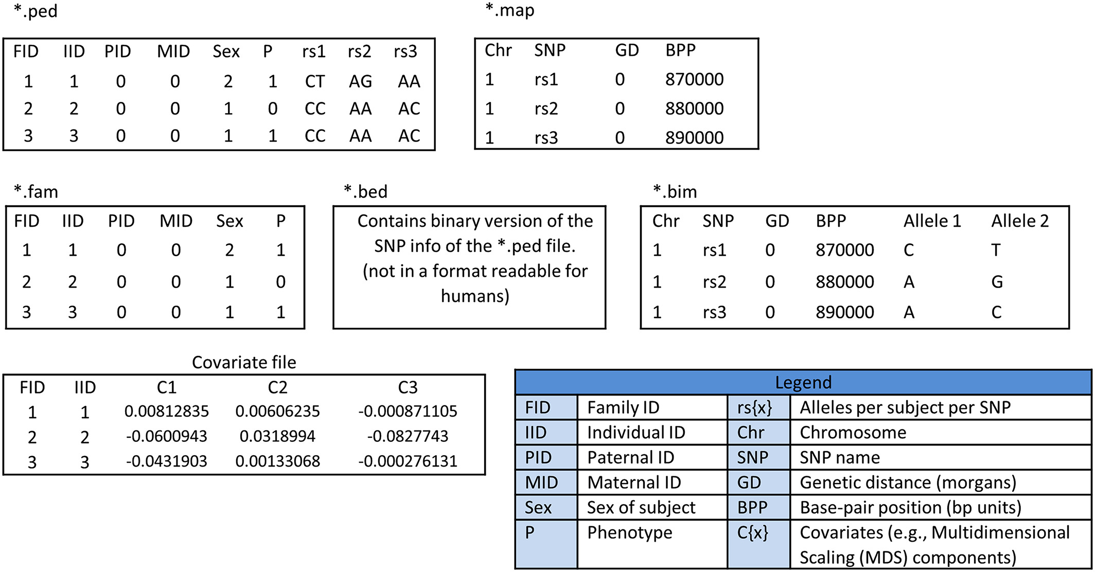
Not all files are used at once, some are results from previous steps during a pipeline, therefore it is important for users to get familiar with the various format types as well as their contents.

Here is a list of terms that are used in GWAS (in alphabetical order):

Term	Definition
Clumping	Identifies and selects the most significant SNP (lowest p-value) in each LD block to reduce correlation while retaining statistically strongest SNPs.
Co-heritability	Measures the genetic relationship between disorders; SNP-based co-heritability represents the proportion of covariance between disorder pairs explained by SNPs.
Gene	A sequence of nucleotides in DNA that codes for a molecule (e.g., a protein).
Heterozygosity	Carrying two different alleles of a specific SNP. High heterozygosity may indicate low sample quality, while low heterozygosity may suggest inbreeding.
Individual-level missingness	The number of SNPs missing for an individual, which may indicate poor DNA quality or technical issues.
Linkage disequilibrium (LD)	Non-random association between alleles at different loci; SNPs are in LD when their allele frequency associations exceed random expectation.
Minor allele frequency (MAF)	Frequency of the least common allele at a specific locus; low MAF SNPs are often excluded due to insufficient statistical power.
Population stratification	Presence of multiple subpopulations in a study; can lead to false positive or masked associations if not corrected for.
Pruning	Selects a subset of SNPs in approximate linkage equilibrium by removing correlated SNPs within a chromosome window; unlike clumping, it does not consider p-values.
Relatedness	Measures genetic similarity between individuals; GWAS assumes unrelated individuals, as relatedness can bias SNP effect estimates.
Sex discrepancy	Difference between reported and genetically determined sex, usually due to sample mix-ups in the lab; identified using SNPs on sex chromosomes.
Single nucleotide polymorphism (SNP)	A variation in a single nucleotide at a specific genome position, typically with two possible alleles (e.g., A vs. T), leading to three possible genotypes (AA, AT, TT).
SNP-heritability	Fraction of phenotypic variance explained by all SNPs in the analysis.
SNP-level missingness	The number of individuals missing information on a specific SNP; high missingness can introduce bias.
Summary statistics	GWAS results including chromosome number, SNP position, SNP ID (rs identifier), MAF, effect size (odds ratio/beta), standard error, and p-value. Often shared openly for research.
The Hardy–Weinberg (dis)equilibrium (HWE) law	Describes allele and genotype frequency stability over generations under ideal conditions (no selection, mutation, or migration). Deviations may indicate genotyping errors or true genetic associations.

---

The publication and tutorial focuses on data from the psychiatric field, specifically focusing on polygenic risk score (PRS) -- an estimate of an individual's genetic predisposition to developing a complex disease. PRS combines the effect sizes of multiple SNPs into a single aggregated score that can be used to predict disease risk, and calculated based on the number of risk variants that a person carries, weighted by SNP effect sizes that are derived from an independent large-scaled discovery GWAS.

As such, the score is an indication of the total genetic risk of a specific individual for a particular trait, which can be used for clinical prediction or screening.

The publication duses data originating from an ethnically homogenous dataset, includeding Utah residents with ancestry from Northern and Western Europe (CEU), as the focus for their work is educational. This sort of study forces Quality Control (QC), sex check, filtering, population stratification, relatedness and heterozygosity checks.

Additionally, the publication does use the 1000 genome data, a large catalogue for research in human variations across all continents. In this tutorial, steps 1 and 2 are already performed, icluding Multidimensional scaling (MDS) of the 1000 genomes data vs the CEU data (steps 1 and 2 are already carried out because downloading and processing the 1000 genome data is extremely time consuming).

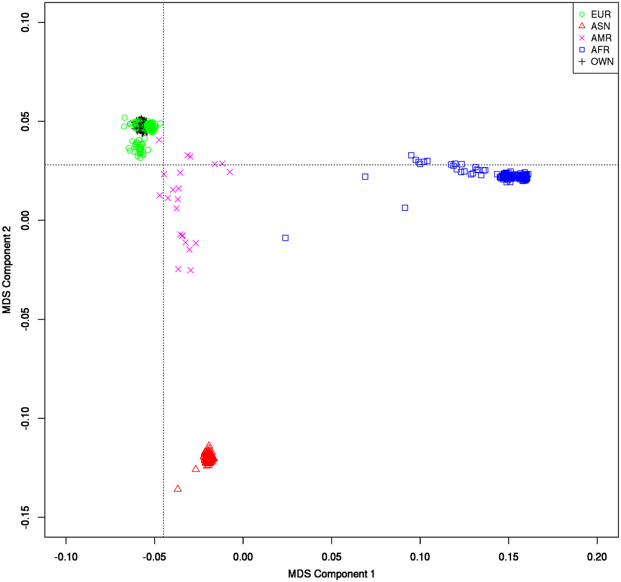
Multidimensional scaling (MDS) plot of 1KG against the CEU of the HapMap data. The black crosses (+ = “OWN”) in the upper left part represent the first two MDS components of the individuals in the HapMap sample (the colored symbols represent the 1KG data

---

This is not set in stone, there isn't a single catch-them-all pipeline. This workshop follows the general outline of the Marees tutorial and from a bird eye view, these are the "steps":

1. Quality Control (QC): essential to produce reliable GWAS outcome (like any other research!).
2. Association Testing: inferring if there is a connection between SNPs to phenotypic traits.
3. Vizualization of results (through a Manhattan plot).

Within QC, the original author performs the following:

• Filtering SNPs & Samples: Removing low-quality data based on missingness, minor allele frequency (MAF), and Hardy-Weinberg Equilibrium (HWE).
• Sex Check: Ensuring consistency between reported and genetic sex.
• Population Stratification: Addressing ethnic differences using Multidimensional Scaling (MDS) and Principal Component Analysis (PCA).
• Heterozygosity Check: Identifying sample contamination.
• Relatedness Check: Removing cryptic relatedness using identity-by-descent (IBD) measures.

Most of these steps are covered in "Step 1" and "Step 2" in the tutorial.

Step 3 focuses on the following:

• Multiple testing correlation. GWAS test millions of SNPs, increasing the risk of false-positive associations. To address this, multiple testing correction methods are applied:
  • Bonferroni Correction: Adjusts the significance threshold by dividing the desired alpha level (e.g., 0.05) by the number of tests performed.
  • False Discovery Rate (FDR): Controls the expected proportion of false positives among the declared significant results, balancing discovery of true associations and control of false positives.
  • Permutation Testing: Involves repeatedly shuffling phenotype labels and recalculating association statistics to empirically determine the distribution of test statistics under the null hypothesis. This method accounts for the correlation structure among SNPs.
• Polygenic Risk Score (PRS) Analysis. PRS aggregates the effects of multiple SNPs to estimate an individual's genetic predisposition to a trait or disease:
  • Calculating PRS: Combining effect sizes from GWAS summary statistics with individual genotype data to compute a risk score.
  • Evaluating PRS Performance: Assessing the predictive power of PRS by comparing risk scores between cases and controls or correlating them with quantitative traits.
  • LD Clumping: A procedure to select independent SNPs by identifying the most significant SNP in each linkage disequilibrium (LD) block, reducing redundancy due to correlated SNPs.
• Generating Manhattan and QQ plots:
  • Manhattan plot: visualizes the p-values of SNP-trait associations across the genome.
    • x-axis = chromosomal position
    • y-axis = −log₁₀(p-value) of p-values, making these look like peaks
    • Uses (previously calculated) Bonferroni correction to help identify significat SNPs.

    

  • QQ (Quantile-Quantile) plot: compares observed p-values from the GWAS to expected p-values under the null hypothesis (no association). It helps detect inflation or systematic bias in the results.
    • x-axis: Expected -log₁₀(p-values) under a uniform distribution.
    • y-axis: Observed -log₁₀(p-values) from the GWAS.
    • Diagonal Line (y = x): Represents what the results should look like under the null hypothesis (i.e., no inflation).
    • how to interpret:
      • Points following the red line = No systematic bias.
      • Upward deviation (left side) = Inflation, meaning an excess of significant SNPs (possible population stratification or confounding).

      

      - Downward deviation (right side) = Deflation, meaning fewer significant SNPs than expected.

      

---

📓 Notebook link: gwas.ipynb (raw)

---

In the tutorial, there are steps that cover both association (--assoc) and logistic (--logistic) tests using plink. Both --assoc and --logistic are association testing methods in PLINK, but they differ in their statistical approach and how they handle covariates.

This method performs a basic association test between each SNP and a binary trait (case-control) using a chi-square test.

How It Works:

• Compares allele frequencies between cases and controls.
• Uses a chi-square test to check if a SNP is significantly associated with the phenotype.
• Does NOT adjust for covariates (e.g., age, sex, population structure).

This method uses logistic regression, which is more advanced than --assoc. It allows the inclusion of covariates (e.g., sex, age, principal components for population structure correction).

How It Works:

• Models the probability of being a case (1) vs. control (0) as a function of SNP genotype and covariates.
• Uses logistic regression equation:

  log(P(Y=1) / 1 - P(Y=1)) = β₀ + β₁x₁ + β₂c₂ + ... + βₙcₙ

• P(Y=1): probability of disease (case status)
• x: SNP genotype (coded as 0, 1, or 2 for allele copies)
• c: covariates (age, sex, principal components)

---

Updated: 03/06/2025 (M. Cosi)

UArizona Data Lab, Data Science Institute, University of Arizona.

CC BY-NC-SA 4.0