An Introduction to Sequence manipulation, Alignment, and Assessment - ua-datalab/Bioinformatics GitHub Wiki
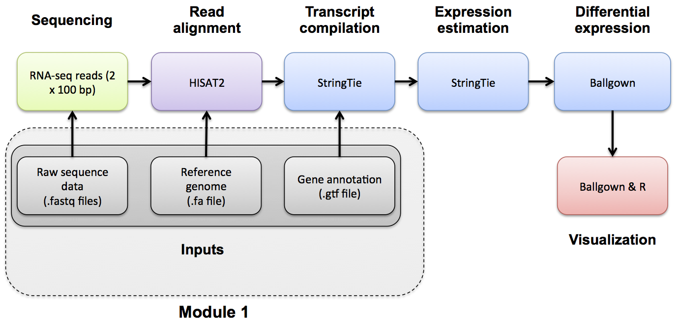
Image credits: Griffith Lab (GitHub, source).
Important
🕐 Schedule
- 2:00pm-2:15pm: Welcome and introdution to topic
- 2:15pm-2:30pm: Handling raw reads
- 2:30pm-2:40pm: Genome indexing and alignments
- 2:40pm-2:50pm: Data formatting
- 2:50pm-3:00pm: Counting features and closing remarks
Important
❗ Requirements
- Basic command line knowledge
- Access to a Terminal
- Unix and Mac users already have access to the Terminal
- Windows users can use either PowerShell or the Windows Subsystem for Linux (WSL)
- A registered CyVerse account (Register for a CyVerse account)
Important
✅ Expected Outcomes
- Hands-on Experience with RNA-seq Data Processing
- Understanding Tools and Methods for alignments and manipulation
This workshop introduces participants to the fundamentals of Sequence manipulation, Alignment, and Assessment by building a streamlined pipeline for transcriptomics. Using M. Musculus (house mouse) as a model organism, attendees will work hands-on with real RNA-seq data, learning to align reads to a reference genome, quantify gene expression. By the end of the session, participants will have a working knowledge of key bioinformatics tools— HISAT2, SAMtools, featureCounts, and DESeq2—and understand how these tools fit together in a typical RNA-seq workflow.
Important
This workshop uses data obtained by the National Center of Biotechnology Information (NCBI).
We are going to be using M. Musculus as the example organism throughout this workshop. All files are made available on CyVerse here or if you are using the command line here: /iplant/home/shared/cyverse_training/datalab/biosciences/m_musculus-seq-tut.
- The M. Musculus genome used will be the GRCm39.
- Curated RefSeq annotations (gff) for the genome can be found in the same location as above.
- RNA-seq data was obtained from the "RNA-seq and Differential Expression" Workshop by Texas A&M HPC group (ACES) for the University of Arizona, first held in April 2024.
Note
Overview of Pipeline As this can be classified as an analysis pipeline, it is important for us to highlight what the major steps are:
[Raw RNA-seq Data QC]
        ↓
[Trimming]
        ↓
[HISAT2 indexing and alignment]
        ↓
[Convert & Sort BAM with SAMtools]
        ↓
[Counting Reads in Features with HTSeq]
In order to get things started:
-
Execute the JupyterLab Bioscience CyVerse App and open the Terminal with 16 CPU cores (min and max) and 16GB RAM memory.
-
Initiate GoCommands, the CyVerse in-house transfer tool using
gocmd init.- Press enter (don't input anything) when propted for iRODS Host, Port, Zone; put your CyVerse username when asked for iRODS Username and your CyVerse password when asked for iRODS Password (Note: you will not see the password being typed as per standard Ubuntu security).
-
Copy the genome files using the following command:
gocmd get --progress /iplant/home/shared/cyverse_training/datalab/biosciences/m_musculus-seq-tut/This will copy:
- Control1_R1.fastq.gz
- Control1_R2.fastq.gz
- GCF_000001635.27_GRCm39_genomic.fna
- GCF_000001635.27_GRCm39_genomic.gff
You are now ready for the workshop!
This section covers popular methods to assess quality of data. FastQC assesses raw data from sequencing runs, useful before an assembly or analysis starts.
Upon obtaining raw sequencing data and before starting your downstream analysis, it is common that at the beginning of your pipeline you run FastQC.
FastQC will help you identify potential issues such as
- Low quality scores at certain positions.
- Adapter contamination.
- Overrepresented sequences.
- GC content anomalies.
The typical workflow including FastQC is the following:
- Run FastQC on the raw reads.
- Review the report for quality issues.
- Perform trimming/cleaning if needed (using tools like Trimmomatic or Cutadapt).
- Optionally, re-run FastQC to confirm the data is clean.
To run fastqc, the commands are
fastqc <sample_data>.fastq -o /path/to/output
Or, if you have multiple samples
fastqc *.fastq -o /path/to/output
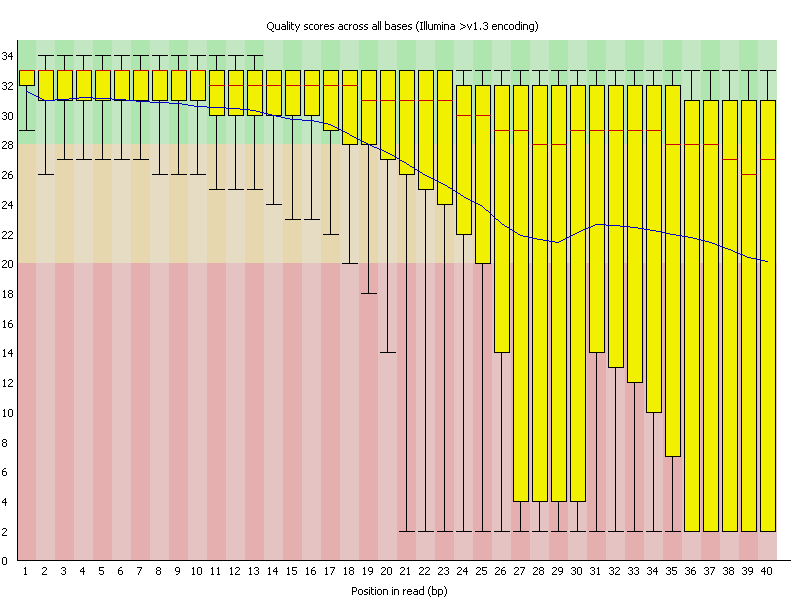
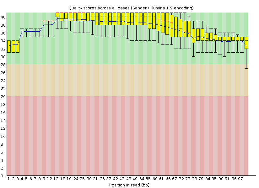
Let's use the figure above to help us understand the output FastQC, called the the Per base sequence quality plot, and it provides the distribution of quality scores at each position in the read across all reads.
- The y-axis gives the quality scores, while the x-axis represents the position in the read.
- The color coding of the plot denotes what are considered high, medium and low quality scores.
- The yellow box represents the 25th and 75th percentiles, with the red line as the median. The whiskers are the 10th and 90th percentiles.
- The blue line represents the average quality score for the nucleotide.
Important
What's the Phred Quality Score?
The y-axis typically represents Phred quality scores, which measure the probability of an incorrect base call. Quality scores are logarithmic and can theoretically go beyond 40. Scores above 40 represent very high confidence in base calls, with probabilities of incorrect base calls being very low (less than 1 in 10,000). Setting the y-axis limit at 40 helps in standardizing the plot and avoiding unnecessary scaling for the majority of sequencing data, where scores often peak around 30 to 40. Scores higher than 40 are relatively rare in most datasets.

Other important results:
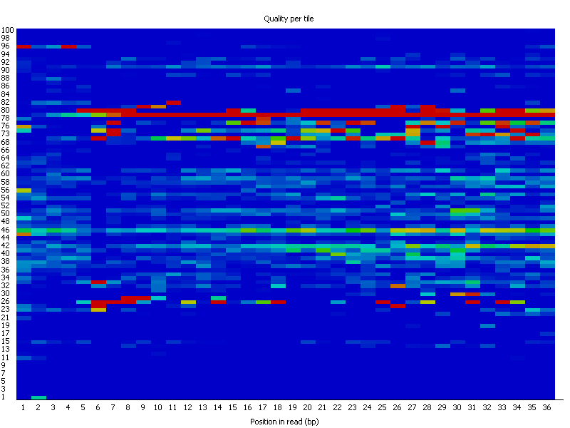
- Per tile sequence quality (only if sequencing was carried out with Illumina): The plot shows the deviation from the average quality for each tile, blue = good, red = bad (heat scale blue to red). Here's an example of a not so great result (source).
- Per sequence quality scores: the average quality score on the x-axis and the number of sequences with that average on the y-axis.
- Per base sequence content: plots out the proportion of each base position in a file for which each of the four normal DNA bases has been called. In a random library you would expect that there would be little to no difference between the different bases of a sequence run, so the lines in this plot should run parallel with each other. Note: this will always fail with RNA-seq data.
- Per sequence GC content: plots the GC distribution over all sequences
- Per base N content: If a sequencer is unable to make a base call with sufficient confidence then it will normally substitute an N rather than a conventional base call. This module plots out the percentage of base calls at each position for which an N was called.
- Sequence Length Distribution: shows the distribution of sequence length.
Execute the command:
fastqc -t 16 -o . Control1_R1.fastq.gz Control1_R2.fastq.gz
The output from FastQC is:
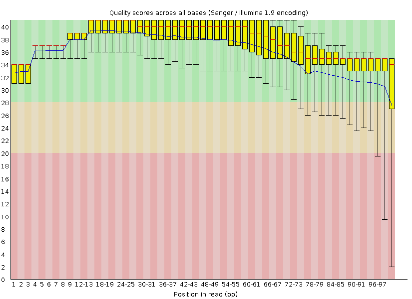
and
How would you interpret these readings?
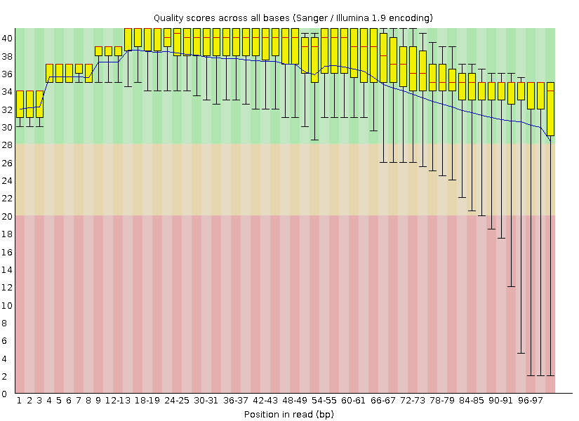
TrimGalore, is a tool for trimming low-quality bases and adapter sequences from high-throughput sequencing reads.
Based on the QC output above, we use TrimGalore's default settings which trims any read that is below length 20. We add the --paired option/flag to only return paired reads.
trim_galore --paired --fastqc Control1_R1.fastq.gz Control1_R2.fastq.gz
The --fastqc option/flag outputs a report we can read in FastQC.
and

Do you think TrimGalore did well? (yes).
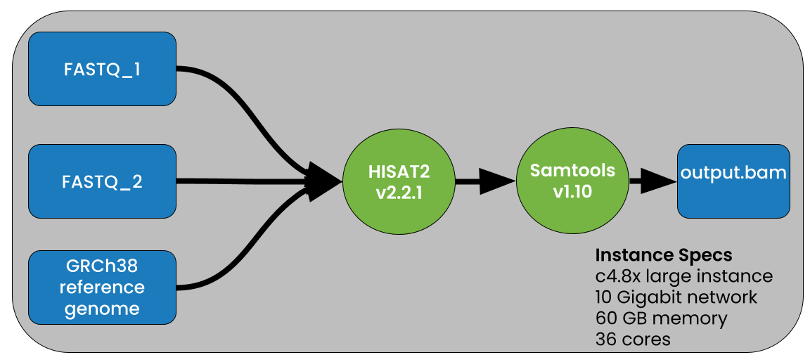
Image source: Petagene. Note: the image above uses the human genome as reference (GRCh38) and specific instant specs.
In this section, we will learn how to process and prepare RNA-seq data for analysis. FASTQ formatted data has been made available on CyVerse (users should first move this data to a local directory). We will then cover how to align these reads to the M. Musculus reference genome using HISAT2, a tool designed for efficient and accurate RNA-seq alignment. Following alignment, we'll use SAMtools to convert the alignment results from SAM to BAM format and sort them, preparing the data for downstream analysis.
HISAT2 is a tool optimized to deal with spliced junctions. It uses the similar algorithms to the BWA aligner, paired with FM-index, a compression algorithm for improved memory efficiency. HISAT2 can handle larger genomes and more complex transcriptomes.
HISAT2 requires an indexed genome, obtainable with a simple synthax:
hisat2-build reference_genome.fa genome_index
Basic synthax:
hisat2 -x genome_index -1 read1.fastq -2 read2.fastq -S output.sam
The options used here are:
-
-x: Specifies the index of the reference genome. -
-1: Specifies the file containing the first reads of paired-end data. -
-2: Specifies the file containing the second reads of paired-end data. -
-S: Specifies the output file in SAM format.
Some other popular options are:
-
-U <single_end_read.fq>: for single end reads -
--dta: Use this option for transcriptome alignments to improve alignments for transcript quantification. -
--rna-strandness: Specify RNA strandness (useFRfor forward,RFfor reverse, orNONEfor no specific strandness). -
--spliced-align: Ensure the aligner considers splicing events. -
--max-intron-len <preferred intron length>: Set the maximum allowed intron length for spliced alignments.
Prior to alignment with HISAT2, we require to index the genome. This can be carried out with the following command synthax. Note, we have added the -p <threads> flag for threads (decreasing the indexing time for larger genomes).
HISAT2 is used to index the model organism of the Mouse first.
hisat2-build -p <threads> <reference-genome.fasta> <reference_index>
Thus, do:
hisat2-build -p 16 GCF_000001635.27_GRCm39_genomic.fna GCF_000001635.27_GRCm39_genomic
This command will build the M. musculus database using 16 threads (time estimation: ~10m).
Note
If you ever need to index larger genomes, do also include the --large-idex flag.
Other flags that are worth using:
-
--ss <splice-sites.txt>: where you point HISAT2 to a txt file where known splice sites are reported. -
--exon <exons.txt>:similar to the splice site option, but for exon information.
Now, you can align your reads. The baseline HISAT2 command for alignment is the following:
hisat2 -x <reference_index> -1 <sample_R1.fastq> -2 <sample_R2.fastq> -S <output.sam>
Then, HISAT2 is used to align our trimmed reads about outputting a SAM file.
 hisat2 -x GCF_000001635.27_GRCm39_genomic -p 16 -1 Control1_R1_val_1.fq.gz -2 Control1_R2_val_2.fq.gz -S Control1.sam
        .
        .
        .
236499 reads; of these:
 236499 (100.00%) were paired; of these:
30736 (13.00%) aligned concordantly 0 times
197200 (83.38%) aligned concordantly exactly 1 time
8563 (3.62%) aligned concordantly >1 times
----
30736 pairs aligned concordantly 0 times; of these:
 3583 (11.66%) aligned discordantly 1 time
----
27153 pairs aligned 0 times concordantly or discordantly; of these:
 54306 mates make up the pairs; of these:
 30660 (56.46%) aligned 0 times
 21188 (39.02%) aligned exactly 1 time
 2458 (4.53%) aligned >1 times
93.52% overall alignment rate
With 93.52% overall alignmet, we score well!
Notice how the output from our most recent alignment is in SAM format. To operate SAM/BAM files, we use SAMtools.
SAMtools is a suite of tools used for manipulating and analyzing files in the SAM (Sequence Alignment/Map) and BAM (Binary Alignment/Map) formats. These formats are commonly used to store alignment data from various sequencing technologies. SAMtools provides a variety of functionalities to process alignment files, including sorting, indexing, and variant calling.
As mentioned before, SAM and BAM files are essentially the same, with one (SAM, Sequence Alignment/Map, larger size) being human readable whilst the other (BAM, Binary Alignment/Map, more compact) is machine readable.
Using SAMtools, we are going to do a few things:
- Convert SAM to BAM. This allows for the downstream analyses to be quicker.
- Sort the reads by genomic coordinates.
- Index the output BAM, allowing fast access to specific regions in the BAM file.
- Check stats.
To convert SAM to BAM, one must do:
samtools view -@ 16 -S -b output.sam > output.bam
The command samtools view converts SAM to BAM. The -S flag specifies the input SAM, -@ <threads> to speed up processing, and -b outputs the BAM file. Notice how the command generates a much smaller file (~3.8GB vs ~700MB).
The next command is the samtools sort command, with -@ <threads> to specify how many threads you want to run it with, -m <memory per thread followed by size (G for GB)>. It's good practice to find ways to multithread your analyses.
samtools sort -@ 16 -m 8G output.bam -o output_sorted.bam
Sorting refers to organizing the alignments in a BAM (or SAM) file based on the genomic coordinates where the reads align to the reference genome. It makes a lot of downstream analyses quicker and more accurate.
Before sorting, the BAM file might look like this:
| Read ID | Chromosome | Position |
|---|---|---|
| R1 | chr1 | 500 |
| R2 | chr2 | 1000 |
| R3 | chr1 | 1500 |
Notice how read ID R2 is on a different chromosome. Post sorting, read ID R3 should be moved closer to R1, as both are on the same chromosome (quicker access downstream).
| Read ID | Chromosome | Position |
|---|---|---|
| R1 | chr1 | 500 |
| R3 | chr1 | 1500 |
| R2 | chr2 | 1000 |
Now you can index your sorted output file; Use -@ <threads> to speed things up and -b to point to the file.
samtools index -@ 16 -b output_sorted.bam
This creates a .bai file, which is your BAM index file.
It is typical to first convert SAM files to BAM as these save space:
samtools view -bS input.sam > output.bam
SAMtools is able to sort SAM/BAM files by the genomic coordinates of the alignments, which is necessary for many downstream analyses:
samtools sort output.bam -o sorted.bam
Typically this is followed by indexing, which creates an index file for BAM files to allow fast access to specific regions of the genome:
samtools index sorted.bam
Returning to our pipeline, we then use SAMtools to sort our alignment and convert SAM into BAM ...
samtools sort -@ 16 -o Control1_sorted.bam Control1.sam
... and index the sorted BAM file.
samtools index Control1_sorted.bam
Note
Notice how we did not use samtools view -bS input.sam > output.bam
This is because certain actions with SAMtools can output directly in the format that we require.
Important
There is more to SAMtools that we are not covering. Users can then create aligment statistics with
samtools flagstat sorted.bam
Or create a pileup file for variant calling:
samtools mpileup -f reference.fasta sorted.bam > variants.bcf
A pileup file is a data format used to represent the sequence coverage at each position in the genome across multiple reads. It provides a compact summary of read alignments and is particularly useful for variant calling and other genomic analyses.
It is useful for the following reasons:
- Coverage Information: shows how many reads cover each position in the genome, helping to identify regions with high or low sequencing coverage.
- Can be used for Base Calls: lists the base calls (nucleotides) observed at each position along with their quality scores.
- Variations: allows for the identification of variations such as SNPs (single nucleotide polymorphisms) and indels (insertions and deletions) by comparing observed bases to the reference genome.
HTSeq-count is a tool for counting the number of reads mapped to specific genomic features (like genes) in RNA-seq data.
We use flags:
-
-r pos: tells HTSeq that the reads in the BAM file are sorted by position (i.e., genomic coordinate), which can be faster if the BAM file is already sorted by position. -
-i gene: sets the feature ID attribute to use for counting ("count the genes for me please!")
htseq-count -r pos -i gene Control1_sorted.bam GCF_000001635.27_GRCm39_genomic.gff > Control1_counts.txt
As it is a txt file, one can open the txt and try to sort through the file themselves, however this is not suggested.
We will be working on this file in the following week.
Updated: 01/30/2025 (M. Cosi)
UArizona Data Lab, Data Science Institute, University of Arizona.

