Arbitrary Wave Generator (AWG) - syue99/Lab_control GitHub Wiki

Introduction

An arbitrary wave generator (AWG) is a key part of our experiment, especially for quantum gate operations. Here at NYU we use Keysight M3201A and Keysight M3201A for our AWG card and this server (keysight_awg) is thus implemented for these two AWG cards. The AWG is used in a similar way as a DDS, as we use it to control the analog signals of our experiment (mainly to AOMs and then modulate our laser light). But the difference between a DDS and an AWG is that it can take in an array of time-series data and output exactly what the array specifies with a time resolution of 1 or 2 ns. On the other hand, a DDS usually takes in inputs of frequency domain parameters such as a frequency, an amplitude, and a phase and outputs a sinewave with these parameters. So an AWG can have more degrees of freedom and is especially helpful when we need complicated pulses that modulate multiple frequencies together (e.g. a Molmer-Sorensen gate).

Running the server

There are multiple ways of running LabRAD server. The easiest is to run this python script itself. At the end of this script, you will see

if __name__ == "__main__":
    from labrad import util
    util.runServer( Keysightawg() )

So if you run this script in the command_line like python PATH-TO\servers\control_instruments\awg\keysightawg.py it will run this chunk of code.

Backgrounds

Given the complicated structures of an awg card, we will give a brief introduction to the AWG hardware, and the corresponding API respectively. We then talk about the functions of the awg server in detail.

Keysight AWG

If you want to learn more about how the awg work in detail (e.g. modulation, trigger, prescale e.t.c), feel free to check out the Keysight user manual section 1.2 9018-04448.pdf.

Hardware Structure and Output modes

As shown by the figure below, a keysight AWG card has four channels of output (x=4). Every output channel consists of a function generator (sine wave, square wave, triangular wave) and a dual AWG generator, and these two generators can either be used separately or together via a fancy digital mixer.

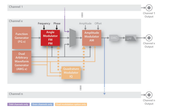
As a result, the awg card supports the following output modes:

1. Function generator (FG) output
2. AWG direct output
3. Amplitude modulation output (use FG for the carrier signal and use AWG for the amplitude)
4. Phase modulation output (Similar to 3, not used by us)
5. IQ modulation output (use FG for the carrier and two AWGs for the modulation)

We use the modes 1,2,3,5 on our servers.

Triggers and Queue

The keysight AWG has an external sma port for the external trigger. It also has digital pins that can be used as external triggers but we haven't played with them yet. So currently we can only trigger one channel without reconfiguration. (The software part for the pins is ready by keysight, we have to test the hardware and make the connection if we want to use this feature later).

The trigger is quite important for us to use the AWG in the experiment. Although in certain experiments (e.g. Rabi scan, Continous Sideband Cooling) we can use a TTL, a switch to control the timing of the AWG, in these scenarios the AWG will just keep playing some waves repeatedly. This cannot work if the waves have time asymmetries, which is the case for all quantum gate experiments (e.g. if we start at the first gate or start with the nth gate leads to different results). As a result, we leave the trigger to the channel that controls the gates, and we will talk in detail in the later sections when talking about the servers.

The trigger is also important as it can be used to control the queue of an AWG. Similar to the pulser, we also first program the waveforms and push the waveforms to chips on the AWG before the experiment so that the FPGA can do the timing during an experiment. As the AWG has a quite large RAM for this (1GB if I remembered correctly), you can push multiple waveforms on the AWG and use triggers to play them one by one. This is particularly useful when we want to play multiple different complicated waveforms in an experiment (e.g. in-circuit measurement but without conditioning logic). Although we did not implement it in our server, it is ready in the API and has been tested.

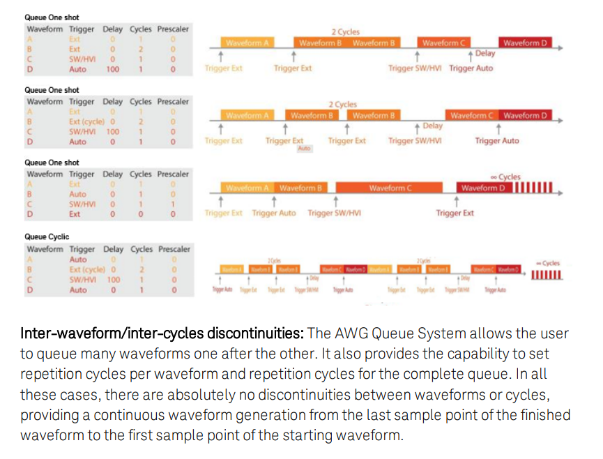
The graph above is an example of a combination of queue and triggers(beside the external trigger we used). Note that for a more complicated queue (e.g. with conditioning logic that Quantum Error Correction needed), we should be able to implement using the HVI packages keysight provided. We didn't play with it as this is an additional software we didn't purchase. Check out 9018-04449.pdf for more.

Prescaling, Sampling Rates and Precisions

The AWG takes a time series signal (even for modulation modes) and outputs an analog signal that follows this waveform. So how is the time units work here? By default, the AWG always plays with the maximal sampling rate. This varies for the two awg cards, as shown by table 1 below.

However, at the same time, we sometimes do not want the AWG to play with the max sampling rate, especially when the signal we played is magnitudes slower than the max sampling rate (e.g. especially in modulation modes). With this prescaling factor, we are able to slow down our sampling rates and thus can save massive data. This would be very useful as it first saves the time for computing and pushing waveforms and also saves the memory so we can have a longer waveform with more gates.

Lastly, the AWG has a precision limit, namely the waveform's precision (amplitudes in Voltage). Again this differs from the two models as shown in table 1. Basically the two models are similar in memory, it is just one has x2 precisions and the other one has x2 sampling rate.

Model	M3201A	M3202A
Sampling Rate	500 MSample/s	1000 MSample/s
Time Interval	2ns	1ns
Precision	16 bit	14 bit

Others

Note that the AWG has some problems with maintaining an accurate phase for a long time(e.g. few seconds), even with it locked with a clock. This limits us from doing deep circuits.

Also, the AWG connects with PC using a PCI-E card and normally does not require a driver. But you have to power up the AWG before the PC is powered up, as otherwise, we find it hard to detect the AWG. Also sometimes the PC just cannot find it, you can restart the PC or check if the PCIE connection is proper or not (the green light would light when the connection is valid)

One last thing is we have experienced two crashes with the AWG. You have to physically restart the AWG to get away from the crash by pressing the power button.

Keysight SD1 (and HVI)

The Keysight SD1 is the official software for their AWGs. We use the python API for the keysight_awg server but it is also nice to first try to use and test the AWG with its default software with their nice GUI. We will briefly introduce the software to make you get familiar with some of the functions and also illustrate an example of a good GUI.

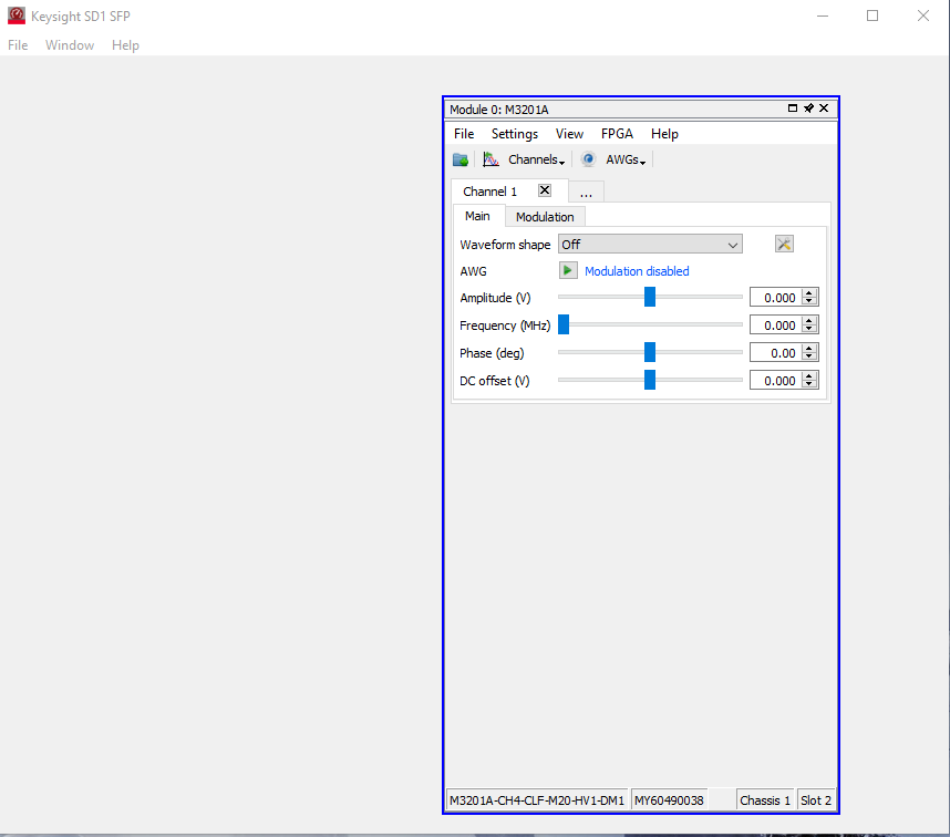
The graph above is the main page for the SD1 software. Every hardware module will result in a pop-up window, as shown in the right part of the graph. In this pop-up window, you can control the waveshape (sin,cos,triangular,awg...) and the corresponding frequency domain parameters (e.g. freq, amp, phase). Note that for AWG waves you can only change the amplitude, all other domain parameters do not affect the output signal. Also, with modulations (set at the top part of the pop-up window), the domain parameters will become the parameters for the carrier signals (and the modulation signal is defined by the AWG signal).

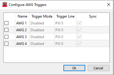
The graph above is the page for setting the triggers. You can set the trigger type, trigger port and etc. here.

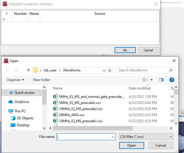
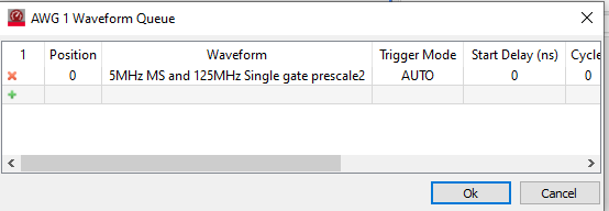
The graph above is the page for pushing the waves. You do that by uploading csv files in this window. Once uploading to the awg memory, you can use the queue system as shown below to determine the cycles, triggers, and orders of how the awg would play the waves.

Also, another big part of the keysight official software is this Keysight Hard Virtual Instrument (HVI) tool. Basically this is a python/graphical programming environment that lets users to program the FPGA inside the AWG. Together with the queue system, one can program more complicated FPGA operations besides playing sequentially or repeatedly. (e.g. if, while logic and ect.) For more information, check out here

Keysight_awg Server

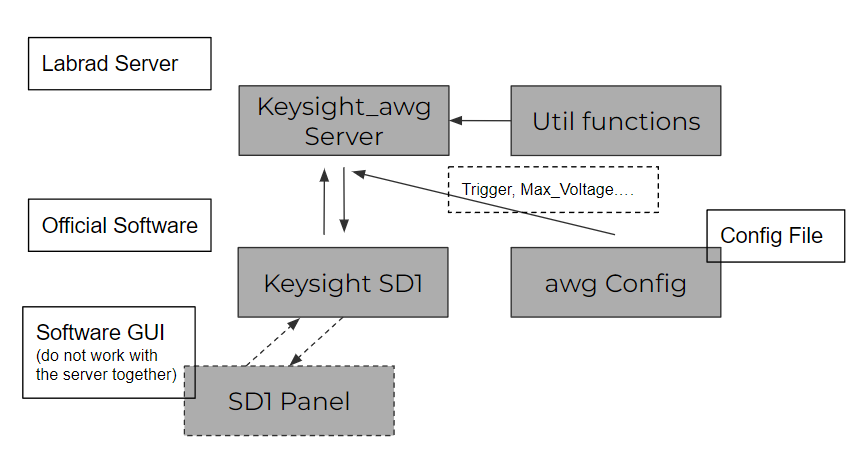
Similar to most other labrad servers, the awg server also calls the python API given by the manufacturer of the instrument (Keysight SD1) to realize different functions we need. As shown by the graph below, the server has a relatively simple structure. There is only one class in keysight_awg.py file that inherits the labrad server class. It gets information from config files in the config folder and gets helper functions (e.g. calculate the normal modes of the ions, get different gates' mathematical functions) from the util subfolder within the server folder.

The AWG server is written in a task-oriented way such that we implement a new function for a task (e.g. play an arbitrary wave, a gate sequence, sideband cooling pulses) when needed. For now, we have the following tasks implemented:

Play a sine wave

We want to use the awg as a DDS. So we use the FG part of the AWG to generate a sine wave. Similar to the pulser, by default when we start the awg server, the awg will play the sine wave according to the default setting specified in the config file. Also, the following methods can be called to control the sine wave output. (the number in the bracket is the method number in the server menus)

1. (1)Amplitude: This method sets the amplitude voltage of the selected channel. It takes in a channel number and a voltage (in the form of labrad units) and can set the amplitude of the sine wave. Note that the voltage cannot be higher than the limit defined by the channel_awg_amp_thres.
2. (2)Frequency: This method sets the frequency of the selected channel. It takes in a channel number and a frequency (in the form of labrad units) and can set the frequency of the sine wave.
3. (3)Phase: This method sets the relative phase of the selected channel. Note that the phases of the four channels are the same initially. It takes in a channel number and a phase (in the form of labrad units) and can set the phase of the sine wave.

Play an arbitrary wave

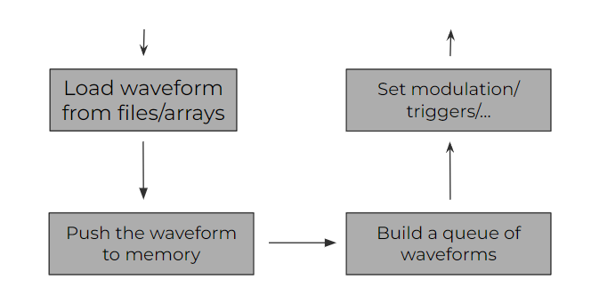
We want to use an arbitrary waveform for various purposes. We use the AWG generator here. More specifically, we use the API to do the following pipeline: load the waveform from an array/a file, then push it to the awg memory, and put it on the first of the queue. A more general pipeline is shown in the graph below, where fancier methods can be implemented based on this pipeline

The following methods can be called to control the awg wave output:

1. (4)AWG Play from File: This method plays a waveform on the selected channel. It takes in a channel number and a file directory (string). After running this method, the awg will load the form and play it repeatedly and immediately.
2. (12)AWG Play from Array: This method plays a waveform on the selected channel. It takes in a channel number and an array. After running this method, the awg will load the form and play it repeatedly and immediately.
3. (5)AWG stop: This method stops the awg signal of the selected channel and switches back to the FG modes (sine wave). It only takes in a channel number

Play waves with Amplitude Modulations:

We want to use the amplitude modulation modes to play the same complicated waveform (e.g. MS gate) as AWG but to save much more data. This is because the AWG mode needs to take in the full-time series waveform in a frequency of ~200MHz, basically hitting the max sampling rate of an awg. On the other hand, using amplitude modulation and using FG as the carrier frequency of ~200 MHz (tunable), we can input a time series waveform in a frequency of ~5MHz (actually the 2xdetuning frequency, see physics of MS-gate for more), which is 40 times less data. The AM modulation follows the same pipeline as the AWG. We just have to set up the FG parameters at the last step and call the modulation mode for the awg. The following methods can be called to control the awg wave output:

1. (6)Arbitrary AM: This method plays an amplitude-modulated(AM) waveform on the selected channel. It takes in a channel number, a file directory for the modulation signal(string), a deviation gain (voltage) that controls the AM signal strength and a carrier freq (frequency) that controls the carrier frequency(on FG). After running this method, the awg will load the form and play it repeatedly and immediately.
2. (7)MS AM: This method plays an amplitude-modulated(AM) waveform of the Molmer-Sorensen interaction on the selected channel. The goal of this method is to just use the experimental parameter fed in to calculate the waveform directly. We do not need to compute the waveform and feed in the actual array or a file, instead we just input the experimental parameters and the method will do the job. A small pipeline is shown below. It takes in a channel number, a deviation gain (voltage), an omega (frequency) which physics-wise is the AOM frequency that bridges the transition frequency and electronic-wise controls the carrier frequency(on FG). After running this method, the awg will first try to load the historically calculated files or calculate the waveform based on the parameters and then play it repeatedly and immediately.
3. (10)Stop AM: This method stops the AM signal of the selected channel and switches back to the FG modes (sine wave). It only takes in a channel number.

Compile a gate sequence

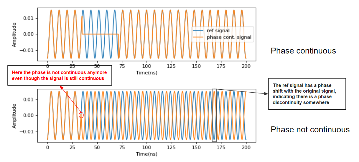
Phase Continouity

One of the most important advantages of AWGs is that we can easily compile a sequence of gates, aka a circuit, and play them on AWGs. This process can be a pain in the butt if we use DDS as the phases of every gate in a circuit should be coherent, as shown by the fig below. The full time-domain control capabilities of AWGs guarantee to respect this continuity if the calculated waveforms are continuous in phase.

Compilation pipeline: Stick and Stack

The compilation pipeline is shown as the graph below: We are given a list of different gates (can be single qubit gates or entangling gates), and we will compute a sequence of pulses that corresponds to the electronic signal we input to AOM to generate the corresponding gates. Note we have to control the start phase of every gate as this phase matters a lot in the interaction. A mismatched phase can generate incorrect interactions (e.g. a single qubit rotation in the Block-sphere around an incorrect axis). Traditionally, this is done by generating one waveform per input gate list. However, this can be very time costly when doing experiments, as it can take more than 50% of the time in a quantum computing experiment. So here we use a stick and stack method, where we guarantee the phase continuity by rounding on the gate time so that the start phase is always continuous with the previous one (unless another interaction is needed, and you change the start phase of the pulse). In this fashion, we can reuse all the historically calculated pulses and just combine them as the gate list requested and achieve orders of magnitudes faster compiling time.

An example: Hamiltonian engineering with 4 ions

The graph below shows an example of a compilation of two different global MS-gates acting on 4 ions (both acting $\sigma_x \sigma_x$ interaction). The MS gate 1 and MS gate 2 are calculated and stick together rather than directly calculated. We make sure the two gates are phase continuous by making sure that every gate will output a small interval $\delta_t$ of 0 signal (as zoomed) so that the next gate will automatically be phase continuous when the phase is set to be 0. We fix the carrier signal to be 125MHz so that we know that $\delta_t< 8ns$, which is a negligible time interval not effecting the experiment. (As this AOM is fixed to be 125MHz, we compensate for the qubit frequency offsets by altering another AOM controlled by DDS).

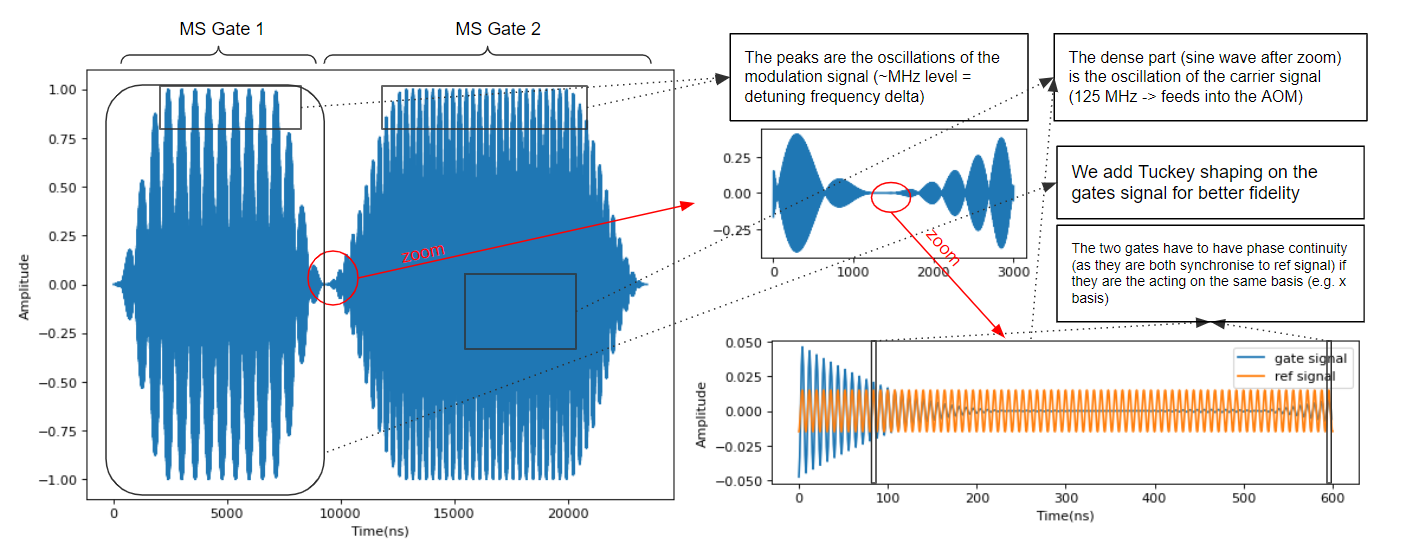
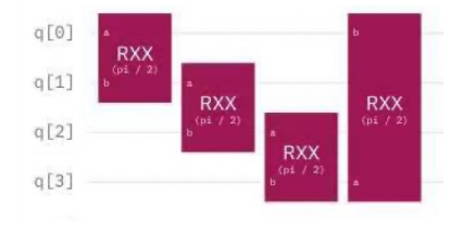
In this real experiment (Hamiltonian engineering of 4 ions), the gate 1 and gate 2 will be stick together in the fashion of layers of gate1,gate2,gate1,gate2...., and using our stick and stack method we save a lot of time from calculating the entire time interval signal (tens of longer than the gate time), and thus making our compilation time under 20 ms for a 180 ms circuit. FYI: the graph below shows the equivalent circuit language of the 1 layer of such interaction (gate1, gate2 just as the graph above), which is composed of 4 entangling gates. So a 180ms (15 layers) circuit corresponds to 60 gates in the circuit language.

IQ modulation

Lastly, in order to further speed up the compilation time. The same feature is implemented with IQ modulation, as you can see from the graph above that the modulation signal is much smaller than the carrier frequency, and we can save a lot of data with IQ modulation. This makes our compilation even faster. For a 10ms circuit with 500 random single and entangling gates (20 us each) that can be a test model for randomized benchmarking, the compilation time is around 300-500ms, which is 4 times faster than the AWG direct output (2s). And this should take only ~20% of the experiment time if we repeat 100 times for every point, which should not be a problem for such experiment.

But note that this feature hasn't been tested on the ions, also it supports less gates (no pulse shaping) though one can later add into the system. (One should compare the signal output on the scope with AWG and IQ modulation and make sure they are the same using the same circuit and then try it on the ions. A tool for the rigol scope has been written and put in the github too, with some explanation ZL-125372298-280822-1553-16590.pdf ).

Gate Compilation Method:

1. (11)Compile Gates: This method uses the direct AWG output/IQ modulation(hasn't tested) to generate a gate sequence with single and two-qubit gates. It takes in a channel number, a Voltage (labrad units), a flag (int) if to use the IQ modulation, a number (int) for the number of repetitions on this circuit (usually the same as the number of repetitions set for the pulser) and a list of gates, for the supported gates can be checked and implemented in the utility/gatedict.py file. Note here every circuit is outputted only if we receive a trigger. So most of the time we configure the trigger to be on the channel that output the gate operations (we refer as the coherent channel)

Generate some specific multitone waveform:

In this section we programmed our AWG to generate various multitone waveforms, mostly for the continuous sideband cooling.

1. (8)Multi Order Sideband Cooling: This method uses the direct AWG output to generate a cooling signal for a multiple tone of multi order center of mass (COM) RSB transitions. It is used for cooling a single ion at high Lamb-Dicke regime but we seldomly use it anymore. It takes in a channel number, a Voltage (labrad units), a frequency for the carrier transition (for AOM to bridge the transition), a COM motional sideband frequency, and a number (int) for the number of orders we want to drive. It will output a multi-tone signal immediately after running and play repeatedly.

2. (9)Multi Ions Sideband Cooling: This method uses the direct AWG output to generate a cooling signal for a multiple tone of multiple motional modes of first order RSB transitions. It is used for cooling a chain of ions at relatively high Lamb-Dicke regime. It takes in a channel number, a Voltage (labrad units), a frequency for the carrier transition (for AOM to bridge the transition), a COM motional sideband frequency, and a number (int) for the number of ions we have in a chain(do not need to be exact). It will output a multi-tone signal immediately after running and play repeatedly.

Resources

One can check User manual for the features Keysight SD1 SDK provides with explanations and Documentation for all the functions in the SDK. Keysight User Manual.pdf