SymPy vs. Mathematica - sympy/sympy GitHub Wiki
 vs.
vs. 
SymPy and Mathematica are Computer algebra systems.
- Computer Algebra System
-
A software program that facilitates symbolic mathematics. The core functionality of a CAS is manipulation of mathematical expressions in symbolic form.
Sympy is a Python library for symbolic computation that aims to become a full-featured computer algebra system and to keep the code simple to promote extensibility and comprehensibility.
SymPy was started by Ondřej Čertík in 2005 and he wrote some code in 2006 as well. In 11 March 2007, SymPy was released to the public. The latest stable release of SymPy is 1.5.1 (5 January 2020). As of 20th of April 2020 there have been over 848 people who contributed at least one commit to SymPy.
SymPy can be used:
- Inside Python, as a library
- As an interactive command line, using IPython
SymPy is entirely written in Python and does not require any external libraries, but various programs that can extend its capabilites can be installed:
- gmpy, Cython --> speed improvement
- Pyglet, Matplotlib --> 2d and 3d plotting
- IPython --> interactive sessions
SymPy is available online at SymPy Live. The site was developed specifically for SymPy. It is a simple web shell that looks similar to iSymPy under the standard Python interpreter. SymPy Live uses Google App Engine as computational backend.
+ +: small library, pure Python, very functional, extensible, large community.
- -: slow, needs better documentation.
Mathematica is a computational software program used in scientific, engineering and mathematical fields and other areas of technical computing.
Mathematica was created by Stephen Wolfram and is developed by Wolfram Research of Champaign, Illinois. The development began in 1986. The first public release was in June 23, 1988. The latest stable release of Mathematica is Mathematica 12.1.0 (March 18, 2020). It is written in Mathematica and C programming languages.
Mathematica has the following features:
- front end with GUI that allows the creation of Notebooks
- development tools (debugger, input completion, automatic syntax coloring)
- command line front end included
- solvers for diophantine equations
Mathematica is proprietary software restricted by both trade secret and copyright law. You can obtain a 15-days trial of Mathematica by signing-up on their official site to download it (1.3 GB). If you want to get Mathematica for more than 15 days, then you can choose one of these versions:
- Professional - $2,495
- Education - $1095
- Student - $140
- Student annual license - $69.95
- Personal - $295.
+ +: full scientific stack, fast, very functional, available in English, Chinese and Japanese.
- -: very large, expensive, not a library, not open source (proprietary).
One of the differences between SymPy and Mathematica is the fact that the latter comes with a GUI that allows the creation of Notebooks. This interface is useful because it allows you to write and run code, display 2d and 3d plots and organize and share your work. However, SymPy can use plotting as well, by installing Pyglet.
| System | Windows | Mac OS X | Linux | BSD | Solaris |
|
|
|
|
|
Yes |
|
|
|
|
|
|
No |
|
|
Sympy is distributed in various forms. It is possible to download source tarballs and packages from the Google Code page but it is also possible to clone the main Git repository or browse the code online. The only prerequisite is Python since Sympy is Python-based library. It is recommended to install IPython as well, for a better experience.
Mathematica can be downloaded from the official site after you sign up. You have to change the execution permissions by writing chmod +x /path/to/Mathematica.sh in a Terminal and execute it (./Mathematica). The installation process is almost automatic.
As you can see in the tables below, there are some differences between the available features in both mathematical systems. SymPy has tensors support, while it is possible to solve diophantine equations in Mathematica.
| System |
Formula editor |
|
|
|
|
|
|
|
|
|
|
|
|
|
| System + |
|
Graph theory |
Number theory |
Quantifier elimination |
Boolean algebra |
Tensors |
|
|
|
|
|
|
|
|
|
|
|
|
|
|
Note
This document contains some examples from Mathematica's documentation and are under a different license than SymPy.
SymPy has a module for tensors that defines indexed objects. However, the module isn't related to mathematical tensors, but it's useful for code generation. Here are some examples:
1) The Indexed class represents the entire indexed object.
           |
        ___|___
       '       '
        M[i, j]
       /   \__\______
       |             |
       |             |
       |     2) The Idx class represent indices and each Idx can
       |           optionally contain information about its range.
       |
3) IndexedBase represents the `stem' of an indexed object, here `M'.
   The stem used by itself is usually taken to represent the entire
   array.
To express the above matrix element example you would write:
In [18]: from sympy.tensor import IndexedBase, Idx

In [19]: from sympy import symbols

In [20]: M = IndexedBase('M')

In [21]: i, j = map(Idx, ['i', 'j'])

In [22]: M[i, j]
Out[22]: M[i, j]
To express a matrix-vector product in terms of Indexed objects:
In [23]: x = IndexedBase('x')

In [24]: M[i, j]*x[j]
Out[24]: M[i, j]⋅x[j]
If an IndexedBase object has no shape information, it is assumed that the array is as large as the ranges of its indices:
In [1]: from sympy.tensor import IndexedBase, Idx

In [2]: from sympy import symbols

In [3]: M = IndexedBase('M')

In [4]: n, m = symbols('n m', integer=True)

In [5]: i = Idx('i', m)

In [6]: j = Idx('j', n)

In [7]: M[i, j].shape
Out[7]: (m, n)

In [8]: M[i, j].ranges
Out[8]: [(0, m - 1), (0, n - 1)]
Mathematica has the Ricci package for tensors:
This is an example of a 2x5x3 tensor:
In[1]:= t = Table[i1 + i2 i3, {i1, 2}, {i2, 5}, {i3, 3}]
Out[1]=
{{{2, 3, 4}, {3, 5, 7}, {4, 7, 10}, {5, 9, 13}, {6, 11, 16}}, {{3, 4, 5}, {4, 6, 8}, {5, 8, 11}, {6, 10, 14}, {7, 12, 17}}}
MatrixForm displays the elements of the tensor in a two-dimensional array.
In[1]:= t = Table[i1 + i2 i3, {i1, 2}, {i2, 5}, {i3, 3}] // MatrixForm
Out[1]=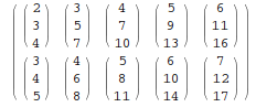
Finding an element in a tensor:
In[1]:= t[ [1, 3, 1] ]
Out[1]= 4
ArrayDepth[t] gives the rank of the tensor. The rank of the tensor is equal to the number of indices needed to specify each element.
In[1]:= ArrayDepth[t]
Out[1]= 3
Diophantine equations provide classic examples of undecidability.
SymPy doesn't have support for solving diophantine equations yet.
Mathematica applies methods based on the latest advances in number theory to solve them. Here are a few examples:
- FindInstance[expr, vars, dom, n] method finds particular solutions to Diophantine equations.
Find an integer solution instance:
In[1]:= FindInstance[x^2 - 3 y^2 == 1 && 10 < x < 100, {x, y}, Integers]
Out[1]=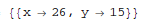
Find several instances:
In[1]:= FindInstance[x^2 - 3 y^2 == 1 && 10 < x < 1000, {x, y}, Integers, 3]
Out[1]=
- Reduce[expr, vars, dom] method is used to perform general reduction of Diophantine equations and inequalities.
Reduce a linear system of equations:
In[1]:= Reduce[2 x + 3 y - 5 z == 1 && 3 x - 4 y + 7 z == 3, {x, y, z}, Integers]
Out[1]= 
Reduce a linear system of equations and inequalities:
In[1]:= Reduce[2 x + 3 y == 4 && 3 x - 4 y <= 5 && x - 2 y > -21, {x, y, z}, Integers]
Out[1]= 
SymPy uses Python constructs only. Here is an example:
>>> 2/7        # Python evaluates this to 0
0

>>> from __future__ import division         # We obtain a different result if we import division from __future__
>>> 2/7
0.285714285714
In Mathematica, the example returns a Rational:
In[1]:= 2/7
Out[1]= 2/7
To obtain a Rational in SymPy, one of these methods must be used:
>>> from sympy import Rational
>>> Rational(2, 7)
2/7

>>> from sympy import S
>>> S(2)/7
2/7
In SymPy, to raise something to a power, you must use **, not ^ as the latter uses the Python meaning, which is xor.
In [1]: (x+1)^2
---------------------------------------------------------------------------
TypeError                                 Traceback (most recent call last)
/home/aoi_hana/sympy/<ipython-input-6-52730bce1577> in <module>()
----> 1 (x+1)^2

TypeError: unsupported operand type(s) for ^: 'Add' and 'int'

In [2]: (x+1)**2
Out[2]:
       2
(x + 1)
However, in Mathematica, ^ means exponentiation and ** is a general associative, but non-commutative, form of multiplication.
In[1]:= (x+1)^2
Out[1]= (x+1)^2

In[1]:= (x+1)**2
Out[1]= (x+1)**2

In[1]:= (1 + x) ** (x + 1) == (x + 1) ** (1 + x)
Out[1]= TrueSymPy
To perform partial fraction decomposition apart(expr, x) must be used. To combine expressions, together(expr, x) is what you need. Here are some examples of these two and other common functions in iSymPy:
In [8]: 1/( (x**2+2*x+1)*(x**2-1) )
Out[8]:
           1
───────────────────────
⎛ 2    ⎞ ⎛ 2          ⎞
⎝x  - 1⎠⋅⎝x  + 2⋅x + 1⎠

In [9]: apart(1/( (x**2+2*x+1)*(x**2-1) ), x)
Out[9]:
      1           1            1            1
- ───────── - ────────── - ────────── + ─────────
  8⋅(x + 1)            2            3   8⋅(x - 1)
              4⋅(x + 1)    2⋅(x + 1)

In [10]: together(1/(x**2+2*x) - 3/(x+y) + 1/(x+y+z))
Out[10]:
x⋅(x + 2)⋅(x + y) - 3⋅x⋅(x + 2)⋅(x + y + z) + (x + y)⋅(x + y + z)
─────────────────────────────────────────────────────────────────
                  x⋅(x + 2)⋅(x + y)⋅(x + y + z)
The evalf() method and the N() function can be used to evaluate expressions:
In [20]: pi.evalf()
Out[20]: 3.14159265358979

In [23]: N(sqrt(2)*pi, 50)
Out[23]: 4.4428829381583662470158809900606936986146216893757
Integrals can be used like regular expressions and support arbitrary precision:
In [24]: Integral(x**(-2*x), (x, 0, oo)).evalf(20)
Out[24]: 2.0784499818221828310
Mathematica
Here are some examples of algebra in Mathematica:
The Apart[expr] method rewrites a rational expression as a sum of terms with minimal denominators.
In[1]:= Apart[1/((x^2+2*x+1)*(x^2-1))]
Out[1]=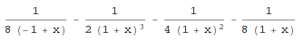
Together[expr] puts terms in a sum over a common denominator, and cancels factors in the result.
In[1]:= Together[1/(x^2+2*x) - 3/(x+y) + 1/(x+y+z)]
Out[1]=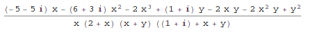
It is possible to evaluate expressions in Mathematica with N[expr]:
In[1]:= N[Pi, 15]
Out[1]= 3.14159265358979

In[2]:= N[Sqrt[2]*Pi, 50]
Out[2]= 4.4428829381583662470158809900606936986146216893757
N() can also compute integrals:
In[1]:= N[Integrate[x^(-2*x), {x, 0, Infinity}], 20]
Out[1]= 2.0784499818221828310SymPy
Limits in SymPy have the following syntax: limit(function, variable, point). Here are some examples:
Limit of f(x)= sin(x)/x as x -> 0
In [20]: from sympy import *

In [21]: x = Symbol('x')

In [22]: limit(sin(x)/x, x, 0)
Out[22]: 1
Limit of f(x)= 2*x+1 as x -> 5/2
In [24]: limit(2*x+1, x, S(5)/2)     # The *S()* method must be used for 5/2 to be Rational in SymPy
Out[24]: 6
Mathematica
Limit[expr, x -> x0] finds the limiting value of expr when x approaches x0.
In[1]:= Limit[Sin[x]/x, x -> 0]
Out[1]= 1

In[1]:= Limit[2*x+1, x -> 5/2]
Out[1]= 6

In[1]:= Limit[(1+x/n)^n, n -> Infinity]
Out[1]= 
The "sqeezing theorem":
In[1]:= Limit[x Sin[1/x], x -> 0]
Out[1]= 0

In[2]:= Plot[{x Sin[1/x], Abs[x], -Abs[x]}, {x, -1, 1}]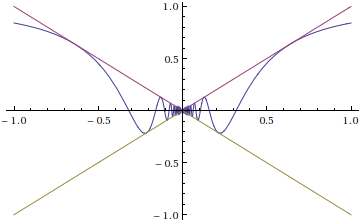
This is the TraditionalForm formatting of Limit[]:
In[1]:= Limit[f[x], x -> x0] //TraditionalForm
Out[1]//TraditionalForm=
SymPy
In [1]: from sympy import *

In [2]: x = Symbol('x')

In [3]: diff(cos(x**3), x)
Out[3]:
    2    ⎛ 3⎞
-3⋅x ⋅sin⎝x ⎠

In [4]: diff(atan(2*x), x)
Out[4]:
   2
────────
   2
4⋅x  + 1

In [6]: diff(1/tan(x), x)
Out[6]:
     2
- tan (x) - 1
─────────────
     2
  tan (x)
Mathematica
The D[expr, var] method from Mathematica is equal to the diff(expr, var)* from SymPy:
In[1]:= D[Cos[x^3], x]
Out[1]= 
In[1]:= D[ArcTan[2*x], x]
Out[1]=
In[1]:= D[1/Tan[x], x]
Out[1]=
This gives the third derivative:
In[1]:= D[x^n, {x, 3}]
Out[1]=
SymPy
The syntax for series expansion is: .series(var, point, order):
In [27]: from sympy import *

In [28]: x = Symbol('x')

In [29]: cos(x).series(x, 0, 14)
Out[29]:
     2    4     6      8       10         12
    x    x     x      x       x          x         ⎛ 14⎞
1 - ── + ── - ─── + ───── - ─────── + ───────── + O⎝x  ⎠
    2    24   720   40320   3628800   479001600

In [30]: (1/cos(x**2)).series(x, 0, 14)
Out[30]:
     4      8       12
    x    5⋅x    61⋅x      ⎛ 14⎞
1 + ── + ──── + ────── + O⎝x  ⎠
    2     24     720
It is possible to make use of series(xcos(x), x)* by creating a wrapper around Basic.series().
In [31]: from sympy import Symbol, cos, series
In [32]: x = Symbol('x')
In [33]: series(cos(x), x)
Out[33]:
     2    4
    x    x     ⎛ 6⎞
1 - ── + ── + O⎝x ⎠
    2    24
Mathematica
Series[f, {x, x0, n}] generates a power series expansion for f about the point x=x0 to order (x-x0)**n.
In[1]:= Series[Cos[x], {x, 0, 14}]
Out[1]=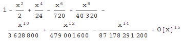
In[1]:= Series[1/Cos[x^2], {x, 0, 14}]
Out[1]=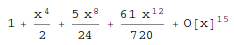
This is the plot of successive series approximations to sin(x)/x:
In[1]:= Plot[Evaluate[Table[Normal[Series[Sin[x]/x, {x, 0, n}]], {n, 20}]], {x, 0, 2 Pi}]
Out[1]=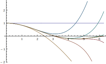
SymPy
The integrals module in SymPy implements methods calculating definite and indefinite integrals of expressions. Principal method in this module is integrate():
- integrate(f, x) returns the indefinite integral

- integrate(f, (x, a, b)) returns the definite integral

SymPy can integrate:
- polynomial functions:
In [6]: from sympy import *

In [7]: import sys

In [8]: from sympy import init_printing

In [9]: init_printing(use_unicode=False, wrap_line=False, no_global=True)

In [10]: x = Symbol('x')

In [11]: integrate(x**2 + 2*x + 4, x)
 3
x     2
── + x  + 4⋅x
3 - rational functions:
In [1]: integrate((x+1)/(x**2+4*x+4), x)
Out[1]:
               1
log(x + 2) + ─────
x + 2- exponential-polynomial functions:
In [5]: integrate(5*x**2 * exp(x) * sin(x), x)
Out[5]:
   2  x             2  x                             x             x
5⋅x ⋅ℯ ⋅sin(x)   5⋅x ⋅ℯ ⋅cos(x)        x          5⋅ℯ ⋅sin(x)   5⋅ℯ ⋅cos(x)
────────────── - ────────────── + 5⋅x⋅ℯ ⋅cos(x) - ─────────── - ──────────
2 2 2 2 - non-elementary integrals:
In [11]: integrate(exp(-x**2)*erf(x), x)
  ___    2
╲╱ π ⋅erf (x)
─────────────
      4
Here is an example of a definite integral (Calculate 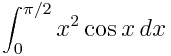 ):
):
In [1]: integrate(x**2 * cos(x), (x, 0, pi/2))
Out[1]:
      2
     π
-2 + ──
     4
Mathematica
To compute integrals in Mathematica, you must use the Integrate[expr, var] || Integrate[expr, {var, lower limit, upper limit}]. Here are some examples:
- polynomial functions:
In[1]:= Integrate[x^2+2*x+4, x]
Out[1]=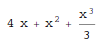
- rational functions:
In[1]:= Integrate[(x+1)/(x^2+4*x+4), x]
Out[1]=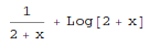
- exponential-polynomial functions:
In[1]:= Integrate[5*x^2*Exp[x]*Sin[x], x]
Out[1]=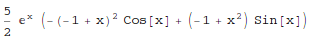
- non-elementary integrals:
In[1]:= Integrate[Exp[-x^2]*Erf[x], x]
Out[1]=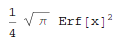
The output of in Mathematica is:
In[1]:= Integrate[x^2*Cos[x], {x, 0, Pi/2}]
Out[1]=
If there is no closed form for a definite integral, then the result is:
In[1]:= Integral[E^-E^x^2, {x, 1, Infinity}]   # Insert the special character Infinity
Out[1]=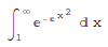
It is possible to get an approximation with NIntegrate:
In[1]:= NIntegrate[E^-E^x^2, {x, 1, Infinity}]
Out[1]= 0.00849838SymPy
In [1]: from sympy import Symbol, exp, I

In [2]: x = Symbol("x")

In [3]: exp(I*2*x).expand()
Out[3]:
 2⋅ⅈ⋅x
ℯ

In [4]: exp(I*2*x).expand(complex=True)
Out[4]:
   -2⋅im(x)                 -2⋅im(x)
ⅈ⋅ℯ        ⋅sin(2⋅re(x)) + ℯ        ⋅cos(2⋅re(x))

In [5]: x = Symbol("x", real=True)

In [6]: exp(I*2*x).expand(complex=True)
Out[6]: ⅈ⋅sin(2⋅x) + cos(2⋅x)
Mathematica
Mathematica has fundamental support for both explicit complex numbers and symbolic complex variables.
It is used in exact and approximate calculations:
In[1]:= Exp[I*2*x]
Out[1]:
In[1]:= ComplexExpand[Exp[I*2*x]]
Out[1]=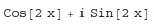
SymPy
trigonometric
In [1]: cos(x-y).expand(trig=True)
Out[1]: sin(x)⋅sin(y) + cos(x)⋅cos(y)

In [2]: cos(2*x).expand(trig=True)
Out[2]:
     2
2⋅cos (x) - 1

In [3]: sinh(I*x**2)
Out[3]:
     ⎛ 2⎞
ⅈ⋅sin⎝x ⎠

In [11]: sinh(acosh(x))
Out[11]:
  _______   _______
╲╱ x - 1 ⋅╲╱ x + 1
zeta function
In [4]: zeta(5, x**2)
Out[4]:
 ⎛    2⎞
ζ⎝5, x ⎠

In [5]: zeta(5, 2)
Out[5]: ζ(5, 2)

In [6]: zeta(4, 1)
Out[6]:
 4
π
──
90
factorials and gamma function
In [7]: a = Symbol('a')

In [8]: b = Symbol('b', integer=True)

In [9]: factorial(a)
Out[9]: a!

In [13]: gamma(b+2).series(b, 0, 3)
Out[13]:
                        2  2             2  2
                       π ⋅b    EulerGamma ⋅b                2    ⎛ 3⎞
1 + b - EulerGamma⋅b + ───── + ────────────── - EulerGamma⋅b  + O⎝b ⎠
                         12          2
polynomials
In [14]: chebyshevt(8,x)
Out[14]:
     8        6        4       2
128⋅x  - 256⋅x  + 160⋅x  - 32⋅x  + 1

In [15]: legendre(3, x)
Out[15]:
   3
5⋅x    3⋅x
──── - ───
 2      2

In [16]: hermite(3, x**2)
Out[16]:
   6       2
8⋅x  - 12⋅x
Mathematica
trigonometric
In[1]:= Expand[Cos[x - y], Trig -> True]
Out[1]=
Cos[x] Cos[y] + Sin[x] Sin[y]

In[1]:= Expand[Cos[2*x], Trig -> True]
Out[1]=
Cos[x]^2 - Sin[x]^2

In[1]:= Sinh[I*x^2]
Out[1]=
FullSimplify[expr] tries a wide range of transformations on expr involving elementary and special functions, and returns the simplest form it finds.
In[1]:= FullSimplify[Sinh[ArcCosh[x]]]
Out[1]=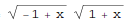
zeta function
In[1]:= Zeta[5, x^2] //TraditionalForm
Out[1]//TraditionalForm=
In[2]:= Zeta[5, 2] //TraditionalForm
Out[1]//TraditionalForm=
In[3]:= Zeta[4, 1]
Out[3]=
The example below returns the Riemann zeta function evaluated at a complex number:
In[1]:= z = 1 + I
In[2]:= N[Zeta[z], 11]
Out[1]=
1 + I
Out[2]=
0.58215805975 - 0.92684856433 I
factorials and gamma function
In[1]:= a!
Out[1]= a!

In[1]:= Table[n!, {n, 10}]
Out[1]=
{1, 2, 6, 24, 120, 720, 5040, 40320, 362880, 3628800}
Gamma[z] is the Euler gamma function  .
.
Series expansion at poles:
In[1]:= Series[Gamma[b + 2], {b, 0, 3}]
Out[1]=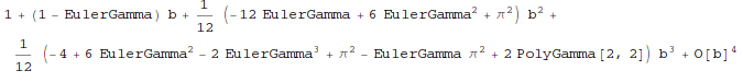
polynomials
ChebyshevT[n, x] gives the Chebyshev polynomial of the first kind Tn(x).
In[1]:= ChebyshevT[8, x]
Out[1]= 1 - 32 x^2 + 160 x^4 - 256 x^6 + 128 x^8

In[2]:= Plot[ChebyshevT[8, x], {x, -1, 1}]
Out[2]=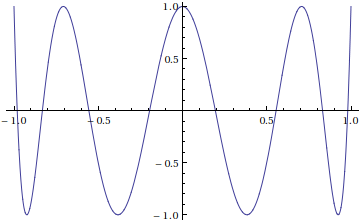
LegendreP[n, z] gives the Legendre polynomial Pn(x):
In[1]:= LegendreP[3, x]
Out[1]=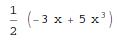
HermiteH[n, x] gives the Hermite polynomial Hn(x):
In[1]:= HermiteH[3, x^2]
Out[1]=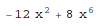
SymPy
In iSymPy:
In [10]: f(x).diff(x, x) + f(x)
Out[10]:
         2
        d
f(x) + ───(f(x))
         2
       dx

In [11]: dsolve(f(x).diff(x, x) + f(x), f(x))
Out[11]: f(x) = C₁⋅sin(x) + C₂⋅cos(x)
Mathematica
Derivative[n1, n2, ...][f] is the general form of the derivative of a function f with one argument. Here is an example:
The derivative of a defined function:
In[1]:= f[x_] := Sin[x^2] + 2*x
        f'[x]
Out[1]=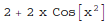
DSolve[eqn, y, x] solves a differential equation for the function y, with independent variable x.
In[1]:= DSolve[y'[x] + y[x] == x, y[x], x]
Out[1]=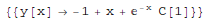
NDSolve[eqns, y, {x, xmin, xmax}] finds a numerical solution to te differential equations eqns.
In[1]:= s = NDSolve[{y'[x] == y[x] Sin[x^2/2 + y[x]], y[0] == 1}, y, {x, 0, 28}]
Out[1]= {{y -> InterpolatingFunction[{{0., 28.}}, <>]}}
The solution can be used in a plot:
In[2]:= Plot[Evaluate[y[x] /. s], {x, 0, 28}, PlotRange -> All]
Out[2]=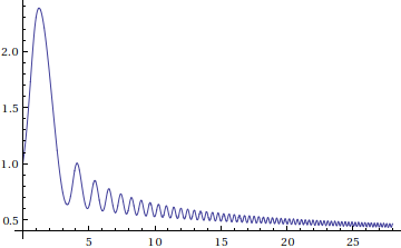
SymPy
In iSymPy:
In [3]: solve(x**3 + 2*x**2 - 1, x)
Out[3]:
⎡            ___      ___    ⎤
⎢      1   ╲╱ 5     ╲╱ 5    1⎥
⎢-1, - ─ + ─────, - ───── - ─⎥
⎣      2     2        2     2⎦


In [5]: solve( [x**2 + 4*y**2 -2, -10*x + 2*y -15], [x, y])
Out[5]:
⎡⎛          ____              ____  ⎞  ⎛          ____              ____   ⎞⎤
⎢⎜  150   ╲╱ 23 ⋅ⅈ   15   5⋅╲╱ 23 ⋅ⅈ ⎟  ⎜  150   ╲╱ 23 ⋅ⅈ   15   5⋅╲╱ 23 ⋅  ⎟⎥
⎢⎜- ─── - ────────, ─── - ──────────⎟, ⎜- ─── + ────────, ─── + ────────── ⎟⎥
⎣⎝  101     101     202      101    ⎠  ⎝  101     101     202      101     ⎠⎦
Mathematica
Solve[expr, vars] attempts to solve the system expr of equations or inequalities for the variables vars.
In[1]:= Solve[x^3 + 2*x^3 == 1, x]
Out[1]=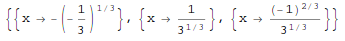
In[1]:= Solve[ {x^2 + 4*y^2-2, -10*x +2 *y -15}, {x, y}]
Out[1]=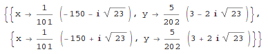
SymPy
In SymPy, matrices are created as instances from the Matrix class:
In [1]: from sympy import Matrix

In [2]: Matrix([ [1, 0 , 0], [0, 1, 0], [0, 0, 1] ])
Out[2]:
⎡1  0  0⎤
⎢       ⎥
⎢0  1  0⎥
⎢       ⎥
⎣0  0  1⎦
It is possible to slice submatrices, since this is Python:
In [4]: M = Matrix(2, 3, [1, 2, 3, 4, 5, 6])

In [5]: M[0:2,0:2]
Out[5]:
⎡1  2⎤
⎢    ⎥
⎣4  5⎦

In [6]: M[1:2,2]
Out[6]: [6]

In [7]: M[:,2]
Out[7]:
⎡3⎤
⎢ ⎥
⎣6⎦
One basic operation involving matrices is the determinant:
In [8]: M = Matrix(( [2, 5, 6], [4, 7, 10], [1, 0, 3] ))

In [9]: M.det()
Out[9]: -10
print_nonzero(symb='x') shows location of non-zero entries for fast shape lookup.
In [10]: M = Matrix(( [2, 0, 0, 1, 0], [3, 5, 0, 1, 0], [10, 4, 0, 1, 2], [1, 6, 0, 0, 0], [0, 4, 0, 2, 2] ))
In [12]: M
Out[12]:
⎡2   0  0  1  0⎤
⎢              ⎥
⎢3   5  0  1  0⎥
⎢              ⎥
⎢10  4  0  1  2⎥
⎢              ⎥
⎢1   6  0  0  0⎥
⎢              ⎥
⎣0   4  0  2  2⎦

In [13]: M.print_nonzero()
[X  X ]
[XX X ]
[XX XX]
[XX   ]
[ X XX]
Matrix transposition with transpose():
In [14]: from sympy import Matrix, I

In [15]: m = Matrix(( (1,2+I), (3,4) ))

In [16]: m
Out[16]:
⎡1  2 + ⅈ⎤
⎢        ⎥
⎣3    4  ⎦

In [17]: m.transpose()
Out[17]:
⎡  1    3⎤
⎢        ⎥
⎣2 + ⅈ  4⎦

In [19]: m.T == m.transpose()
Out[19]: True
Mathematica
You can create a matrix in Mathematica with the use of lists. The result can be displayed in matrix notation with MatrixForm.
In[1]:= mat = { {1, 0, 0}, {0, 1, 0}, {0, 0, 1} }
Out[1]= {{1, 0, 0}, {0, 1, 0}, {0,

In[2]:= mat //MatrixForm
Out[2]//MatrixForm=
Det[m] gives the determinant of the square matrix m.
In[1]:= Det[ { {2, 5, 6}, {4, 7, 10}, {1, 0, 3} } ]
Out[1]= -10
Matrix transposition is with Transpose[m]:
In[1]:= Transpose[ { {1, 2+I}, {3, 4} } ] //MatrixForm
Out[1]//MatrixForm=
SymPy
The geometry module can be used to create two-dimensional geometrical entities and query information about them. These entities are available:
- Point
- Line, Ray, Segment
- Ellipse, Circle
- Polygon, RegularPolygon, Triangle
Check if points are collinear:
In [37]: from sympy import *

In [38]: from sympy.geometry import *

In [39]: x = Point(0, 0)

In [40]: y = Point(3, 1)

In [41]: z = Point(5, 5)

In [42]: Point.is_collinear(x, y, z)
Out[42]: False

In [43]: Point.is_collinear(x, z)
Out[43]: True
Segment declaration, slope, length, midpoint:
In [1]: import sympy

In [2]: from sympy import Point

In [3]: from sympy.abc import s

In [4]: from sympy.geometry import Segment

In [5]: Segment( (1, 2), (2, -3))
Out[5]: ((1,), (2,))

In [6]: s = Segment(Point(4, 3), Point(1, 1))

In [7]: s
Out[7]: ((1,), (4,))

In [8]: s.points
Out[8]: ((1,), (4,))

In [9]: s.slope
Out[9]: 2/3

In [10]: s.length
Out[10]:
  ____
╲╱ 13

In [11]: s.midpoint
Out[11]: (5/2,)
Mathematica
Point[coords] is a graphics primitive that represents a point.
In[1]:= p = Table[{t, Cos[t]}, {t, 0, 2 Pi, 2 Pi/10}];
    {Graphics[{PointSize[Tiny], Point[p]}],
    Graphics[{PointSize[Small], Red, Point[p]}],
    Graphics[{PointSize[Medium], Blue, Point[p]}],
    Graphics[{PointSize[Large], Green, Point[p]}]}
Out[1]=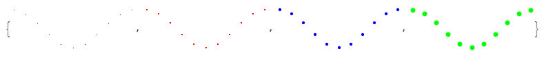
Points on the unit sphere:
In[1]:= Block[{sp = Normalize /@ RandomReal[{-1, 1}, {3*10^4, 3}]}, Graphics3D[{Point[sp, VertexNormals -> sp]}]]
Out[1]=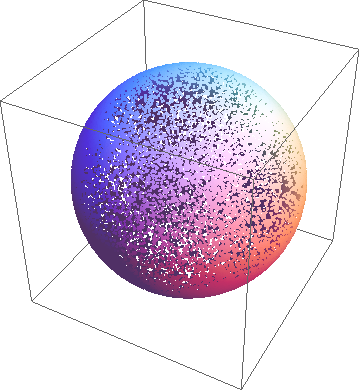
This is a complete graph with 10 vertices:
In[1]:= p = Table[{Cos[2 n Pi/9], Sin[2 n Pi/9]}, {n, 0, 9}];
In[2]:= Graphics[{Opacity[0.7], Blue, Line[Tuples[p, 2]], Red, PointSize[0.03], Point[p]}]
Out[2]=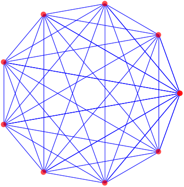
SymPy
Using the .match method and the Wild class you can perform pattern matching on expressions. The method returns a dictionary with the needed substitutions. Here is an example:
In [11]: from sympy import *

In [12]: x = Symbol('x')

In [13]: y = Wild('y')

In [14]: (10*x**3).match(y*x**3)
Out[14]: {y: 10}

In [15]: s = Wild('s')

In [16]: (x**4).match(y*x**s)
Out[16]: {s: 4, y: 1}
SymPy returns None if the match is unsuccessful:
In [19]: print (x+1).match(y**x)
None
Mathematica
Cases[list, form] gives the elements of list that match form.
In this example, Cases() returns the elements of the list which match the pattern x ^ _.
In[1]:= Cases[{1, 0, x^2, x^10, x/4, x^3}, x^_]
Out[1]=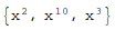
To return only the part of the expression that matches the pattern, chars_ must be used:
In[1]:= Cases[ {10*x^3}, n_*x^3 -> n ]
Out[1]=
Cases() returns {} when the match is unsuccessful.
SymPy
There are many ways of printing mathematical expressions. Two of the most common methods are:
- Standard printing
- Pretty printing using the pprint() function
- Pretty printing using the init_printing() method
Standard printing is the return value of str(expression):
>>> from sympy import Integral   # Python session
>>> from sympy.abc import c
>>> print c**3
c**3
>>> print 2/c
2/c
>>> print Integral(c**2+2*c, c)
Integral(c**2 + 2*c, c)
Pretty printing is a nice ascii-art printing with the help of a pprint function.
In [1]: from sympy import Integral, pprint   # IPython session (pprint enabled by default)

In [2]: from sympy.abc import c

In [3]: pprint(c**3)
 3
c

In [4]: pprint(2/c)
2
─
c

In [5]: pprint(Integral(c**2+2*c, c))
⌠
⎮ ⎛ 2      ⎞
⎮ ⎝c  + 2⋅c⎠ dc
⌡
However, the proper way to set up pretty printing in SymPy is to use init_printing(pretty_print=True, order=None, use_unicode=None, wrap_line=None, num_columns=None, no_global=False, ip=None):
>>> from sympy import init_printing
>>> init_printing(use_unicode=False, wrap_line=False, no_global=True)
>>> from sympy import Integral, Symbol
>>> x = Symbol('x')
>>> Integral(x**3+2*x+1, x)
  /
 |
 | / 3          \
 | \x  + 2*x + 1/ dx
 |
/
>>> init_printing(pretty_print=True)
>>> Integral(x**3+2*x+1, x)
⌠
⎮ ⎛ 3          ⎞
⎮ ⎝x  + 2⋅x + 1⎠ dx
⌡
Mathematica
The following three printing methods are commonly used in Mathematica to format both input and output:
- TraditionalForm method
- StandardForm or InputForm methods
- Print[expr] function
The sum of 1/n^Sqrt[2] from n=1 to n=Infinity is Zeta[Sqrt[2]]:
In[1]:= Sum[1/m^Sqrt[2], {n, 1, Infinity}]
Out[1]=
To convert the above output in the traditional mathematic form, then the TraditionalForm method is used:
In[1]:= Sum[1/n^Sqrt[2], {n, 1, Infinity] // TraditionalForm
Out[1]//TraditionalForm=
StandardForm and InputForm work in reverse.
InputForm is used to find out how to type an expression into Mathematica:
In[1]:= |input1| // InputForm
Out[1]//InputForm=
Zeta[Sqrt[2]]
The StandardForm is more compact than InputForm and is similar to the pprint() method from SymPy.
In[1]:= |input2| // StandardForm
Out[1]//StandardForm=
The Print[expr] function prints expr as output.
In[1]:= Print[x + y]; Print[a + b]
Out[1]=
x + y
a + b
Print the first three prime numbers:
In[1]:= Do[Print[Prime[p]], {p, 3}]
Out[1]=
2
3
5SymPy
Pyglet is required to use the plotting function of SymPy in 2d and 3d. Here is an example:
>>> from sympy import symbols, Plot, cos, sin
>>> x, y = symbols('x y')
>>> Plot(sin(x*10)*cos(y*5) - x*y)
[0]: -x*y + sin(10*x)*cos(5*y), 'mode=cartesian'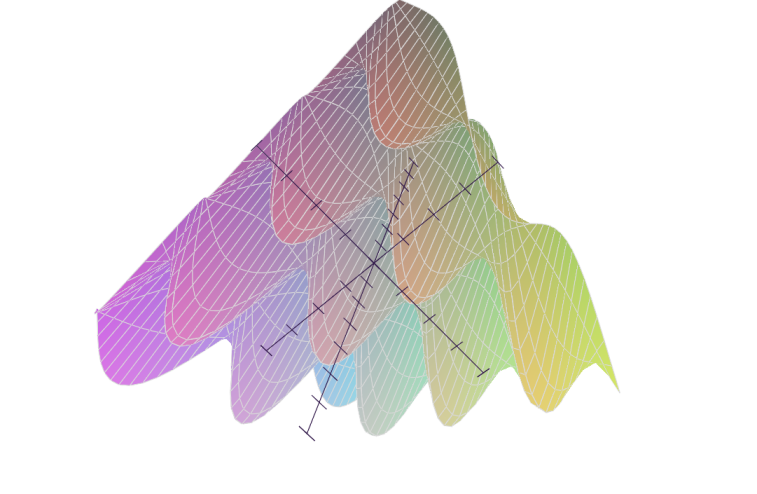
In[1]: Plot(cos(x*y*10))
Out[1]: [0]: cos(10*x*y), 'mode=cartesian'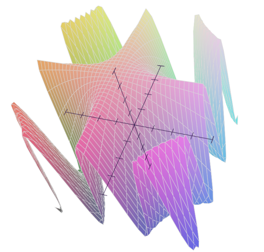
Mathematica
There are three types of plotting in Mathematica:
- Plot[f, {x, xmin, xmax}]
- Plot3D[f, {x, xmin, xmax}, {y, ymin, ymax}]
- RegionPlot[pred, {x, xmin, xmax}, {y, ymin, ymax}]
Here are some examples of the plotting functions:
Plot
Eigenfunctions in a potential well:
In[1]:= f[n_, x_] := Abs[((1/Pi)^(1/4) HermiteH[n, x])/(E^(x^2/2) Sqrt[2^n n!])]^2;
In[2]:= Plot[Evaluate@Append[Table[f[n, x] + n + 1/2, {n, 0, 10}], x^2/2], {x, -5, 5}, Filling -> Table[n -> n - 1/2, {n, 1, 11}]]
Out[2]=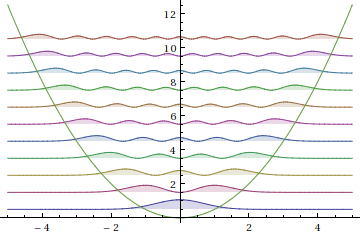
RegionPlot
Exclusive OR of five disks:
In[1]:= disk[m_, n_] := Block[{x0 = 1/2 Cos[m 2 Pi/n], y0 = 1/2 Sin[m 2 Pi/n]}, (x - x0)^2 + (y - y0)^2 < 1]
In[2]:= disk[n_] := Apply[Xor, Table[disk[m, n], {m, 0, n - 1}]]
In[3]:= RegionPlot[disk[5], {x, -2, 2}, {y, -2, 2}, FrameTicks -> None]
Out[3]=
Plot3D
Plot of Cos[x*y*10] in Mathematica:
In[1]:= Plot3D[Cos[x*y*10], {x, -1, 1}, {y, -1, 1}]
Out[1]=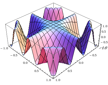
A function with restricted domain and different coloring:
In[1]:= Plot3D[{x^2 + y^2, -x^2 - y^2}, {x, -1, 1}, {y, -1, 1}, RegionFunction -> Function[{x, y, z}, x^2 + y^2 <= 4], BoxRatios -> Automatic, ColorFunction -> Hue, MeshShading -> {{Automatic, None}, {None, Automatic}}]
Out[1]=
There are more plotting methods, such as ListPointPlot3D (Four conical spirals example):
In[1]:= ListPointPlot3D[Table[Table[(4 Pi - t) {Cos[t + s Pi/2], Sin[t + s Pi/2], 0} + {0, 0, 2 t}, {t, 0, 4 Pi, .1}], {s, 4}], Filling -> Bottom, ColorFunction -> "Rainbow", BoxRatios -> Automatic, FillingStyle -> Directive[LightGreen, Thick, Opacity[.1]]]
Out[1]=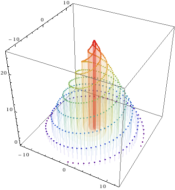
SymPy aims to be a lightweight normal Python module so as to become a nice open source alternative to Mathematica. Its goal is to be reasonably fast, easily extended with your own ideas, be callable from Python and could be used in real world problems. Another advantage of SymPy compared to Mathematica is that since it is written in pure Python (and doesn't need anything else), it is perfectly multiplatform, it's small and easy to install and use.
You can choose to use either SymPy or Mathematica, depending on what your needs are. For more information you can go to the official sites of SymPy and Mathematica.