Nodes - sufiyan63/SAP-Hana-Cloud GitHub Wiki
- Intersect Node
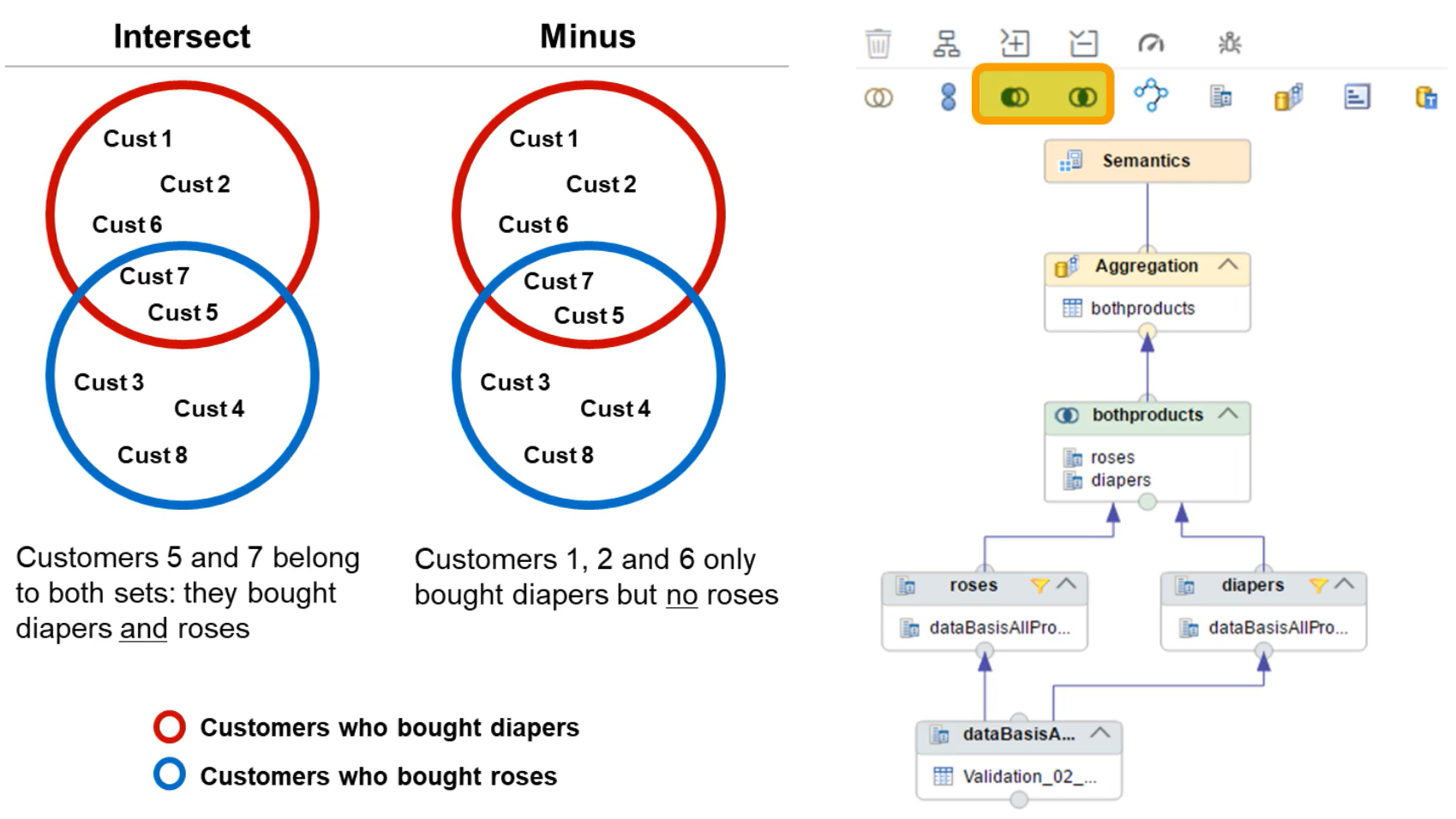
- The intersect node is used to select the rows from one data source that also appear in another data source. You choose the columns on which the intersection check is made.
- works on entire data sets
- We need to map to the same columns in output table eg. projection_A has REGION and CATEGORY. Projection_B has REGION and CATEGORY. We have only one REGION and CATEOGRY in output table projecting from two views
- The difference between INNER JOIN and INTERSECT in SQL lies in their purpose and behaviour when handling sets of data:
-
Data Relationship:
INNER JOIN
explicitly connects tables based on a relationship (e.g., foreign key), whileINTERSECT
works on entire result sets and does not require table relationships. -
Output Scope:
INNER JOIN
outputs columns from both tables, whereasINTERSECT
only provides the intersecting rows matching all selected columns. SELECT ID, Name FROM TableA INTERSECT SELECT ID, Name FROM TableB;- This query fetches rows (ID and Name) that are common to both
TableA
andTableB
. - Minus node
- The minus node is used to select rows that appear in one data source but not another. Again, you choose the columns on which the minus check is made.
- For the Minus node, the data sets are considered based on their order in the list of data sources for the node. Therefore, the output contains items from the FIRST data source that are NOT in the SECOND data source. In SAP HANA Cloud, it is possible to change the order of the data sources: just right-click on the Minus node and choose Switch Order.
- There are two data sets – data set A and data set B
- Dataset A contain all the regions
- Dataset B contain only US region
- If I add these two data source in minus node then the output is the data set containing all regions except US region
- Semantics node
- This node is used to define enrichments to the final results set, such as adding currency information to measures, or apply masking rules to cover up sensitive parts of a data
- it is already present and will always be the top node
- Display separately the view-global information, such as view properties (including caching and snapshots queries),
- In this node, you assign semantics to each column in order to define its behaviour and meaning. This is important information used by consuming clients so that they are able to display and process the columns appropriately.
- One of the most important and mandatory settings for each column is its column type. You can choose between attribute or measure
- Private tab contains the output column you created from the previous node
- Shared tab will show all the outputs from other dimension views
- Hiding a column – This can be used if a column is only used in a calculation, or is an internal value that should not be shown, for example, hiding the unhelpful product id when we have assigned a description column that should be shown in its place.
-
Semantics type
- you can also optionally assign to each column
- For example, if you define a column as a date semantic type, the front-end application can format the value with separators rather that a simple string. The key point is that it is the responsibility of the front-end application or consuming client to make use of this additional information provided by the semantic type.
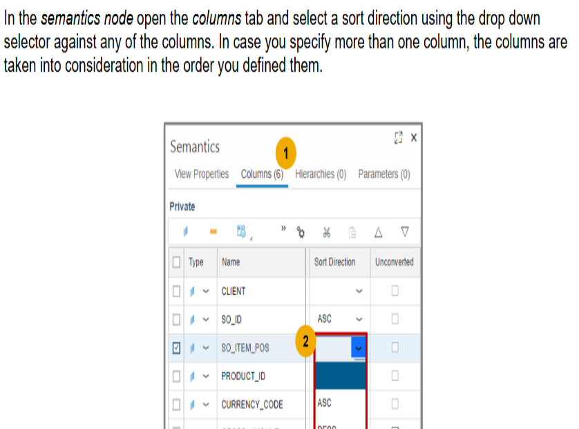
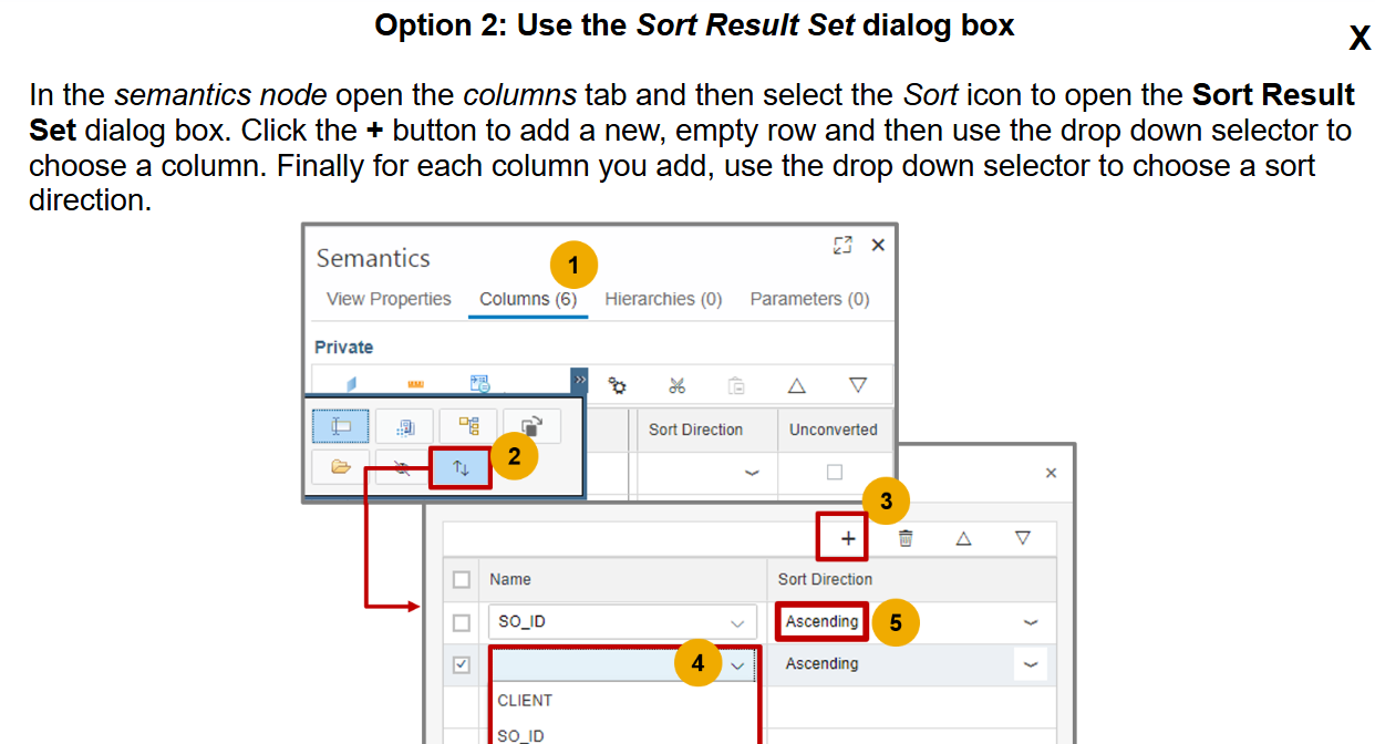
- Sort Direction Property
- Suppose a calculation view (a type of database view) is designed to sort data by two columns, say
SO_ID
first and thenPRODUCT_ID
. - If a client (like a front-end tool) sends a query that only specifies sorting by
PRODUCT_ID
, the database might not maintain the original sorting order defined in the calculation view (SO_ID
thenPRODUCT_ID
). -
Result Set Order: As a result, the data might not be sorted as expected. To ensure the data is sorted by both
SO_ID
andPRODUCT_ID
, the client query must explicitly include both columns in theORDER BY
clause. - In essence, to achieve the desired sorting order, the client query needs to match the sorting columns defined in the calculation view. Does that help clarify things?
- the client query will take priority. If the client query specifies sorting only by
PRODUCT_ID
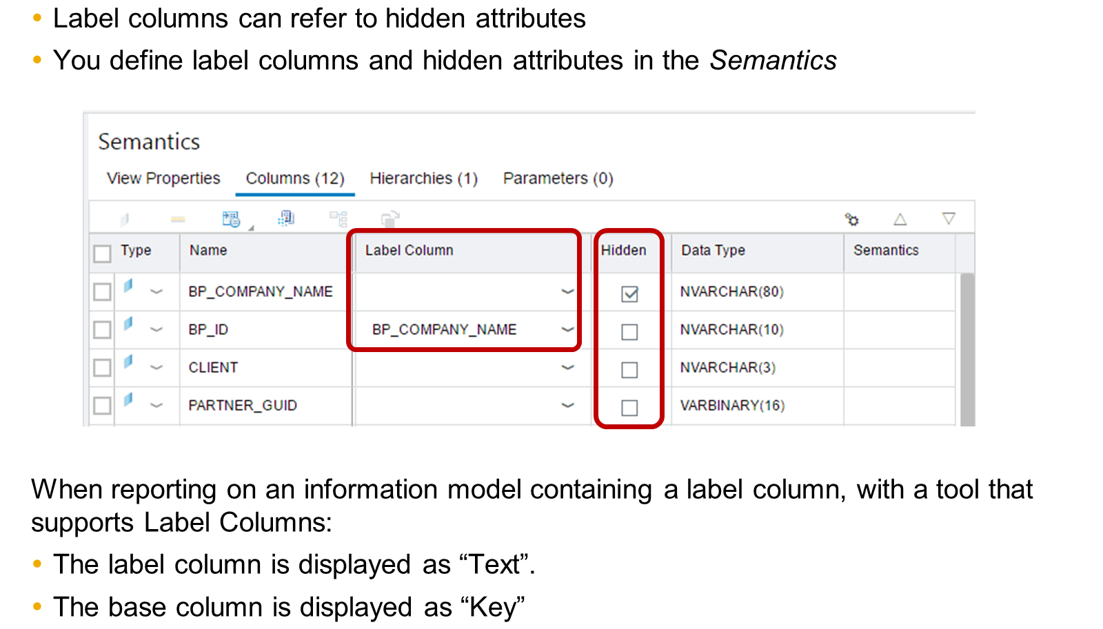
- Label Column Field
- Assigning a description column to another column – for example, assigning the product id column to a product description column so that a user sees a value which is more meaningful.
- navigate to the "Semantics" node within the view editor, select the column you want to describe, then in the properties panel, use the "Label Column" field to choose the column containing the description text
- Null Values
- Columns, both attributes and measures can contain undefined values or null values. You can handle such cases by defining default values that replaces the null values in reporting tools.
- For example, you can replace the column values that would usually appear with the null value representation of '?' with a default value 'Null', or 'Empty' or with any other user defined value that you prefer.
- Select the Semantics node
- Choose the Columns tab
- Select a measure or attribute
- Select the 'Null Handling' checkbox
- Optionally, in the Default Value text field, provide a default value
- If you have enabled null handling for columns and if you have not provided any default value, then the tool considers the integer 0 as the default value for columns. However, for columns of data type NVARCHAR, if you have not defined a default value after enabling null handling, the tool displays an empty string, (which means blank), as the default value.
- Private and Shared Columns
- the Columns tab of the Semantics node separates columns into two categories
- Private
- Private columns are columns that are defined inside the calculation view itself. These can be measures or attributes. You have full control over these columns.
- Shared
- Shared columns are columns that are defined "externally", in one or more dimension calculation views that are referenced by your cube with star join calculation view. On these columns, you have logically less control, because they are potentially "shared" with another cube with a star join calculation view. Still, you can hide some of these columns to only keep the ones that you need.
- Regarding the shared columns, their Name and Label properties cannot be changed, compared with a private column, but you can define an Alias Name and an Alias Label. Moreover, providing Alias Names is mandatory if column names from the underlying dimension calculation views conflict with each other or conflict with the private column names.
-
Properties of Views – General
- Data Category ⇒ For calculation views, this determines whether the view supports multidimensional reporting.
- Type ⇒ Standard or Time
- Default Client ⇒ Defines how to filter data by SAP CLIENT (aka MANDT).
- Apply Privileges ⇒ Specifies whether analytic privileges must apply when executing a view (SAP Business Application Studio for SAP HANA modeling supports SQL analytic privileges only).
- Enable Hierarchies for SQL access ⇒ In a calculation view of type CUBE with star join, determines whether the hierarchies defined in shared dimension views can be queried via SQL.
- End-User View ⇒ Specify whether to offer this calculation view as a source to reporting tools.
-
Properties of Views – Advanced
- Propagate instantiation to SQL Views ⇒ If the calculation view is referenced by an SQL view or a Core Data Services (CDS) view, it determines whether the calculation view must be instantiated. For example, it prunes columns that are not selected by the previous queries) or executed exactly as it is defined.
- Analytic View Compatibility Mode ⇒ If this setting is activated, the join engine ignores joins with cardinality n..m defined in the star join node when no column at all is queried from one of the two joined tables.
- Ignore Multiple Outputs For Filter ⇒ Optimization setting to push down filters even if a node is used in more than one other node.
- Pruning Configuration Table ⇒ Identifies which table contains the settings to prune Union nodes.
- Execute in ⇒ Determines whether the model must be executed by the SQL engine or column engine.
- Execution Hints ⇒ This property is used to specify how the SAP HANA engines must handle the calculation view at runtime.
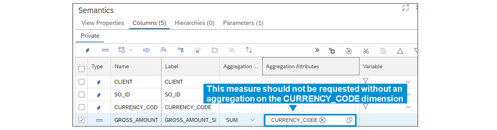
- Aggregation Attributes
- For each measure of the calculation view, you can define one or several attributes that should be kept when aggregating data.
- The information entered in the Semantics is meant to be used by reporting tools
- The setting defined in the Semantics has no influence on the way aggregations are executed by the calculation engine. Besides, it does not prevent the execution of a query that might return inconsistent data because an aggregation attribute needed for a given column has not been included.
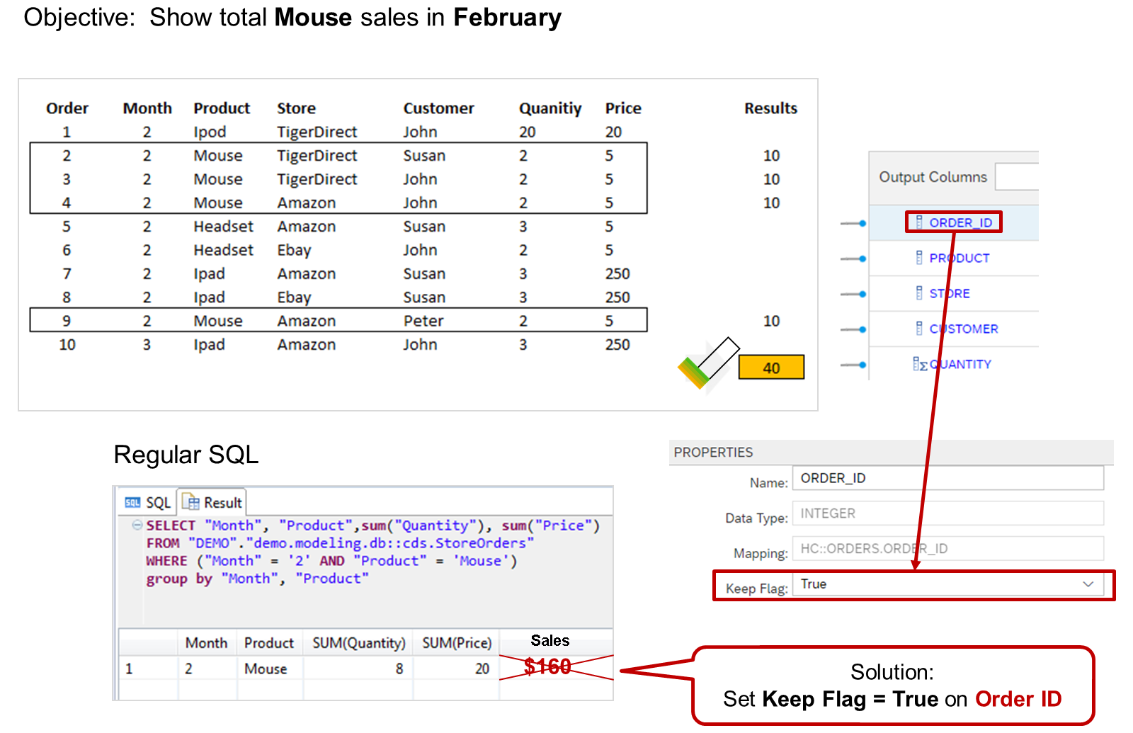
- Keep Flag
- Setting the Keep Flag property to true for the Order ID column forces the calculation to be triggered at the relevant level of granularity, even if this level is not the grouping level defined by the client query.
- The Keep Flag option can also be defined on the shared columns in the Star Join node of a CUBE with Star Join calculation view
- for any calculations column ⇒ multiplication should happen first and then summation or subtraction
- To include a lower level of granularity
- In the aggregation node you need to enable the keep flag property for Primary ID like order_id, employee_id
- By doing this you get accurate results ⇒ For each order_id we multiply the price and quantity and then sum take place
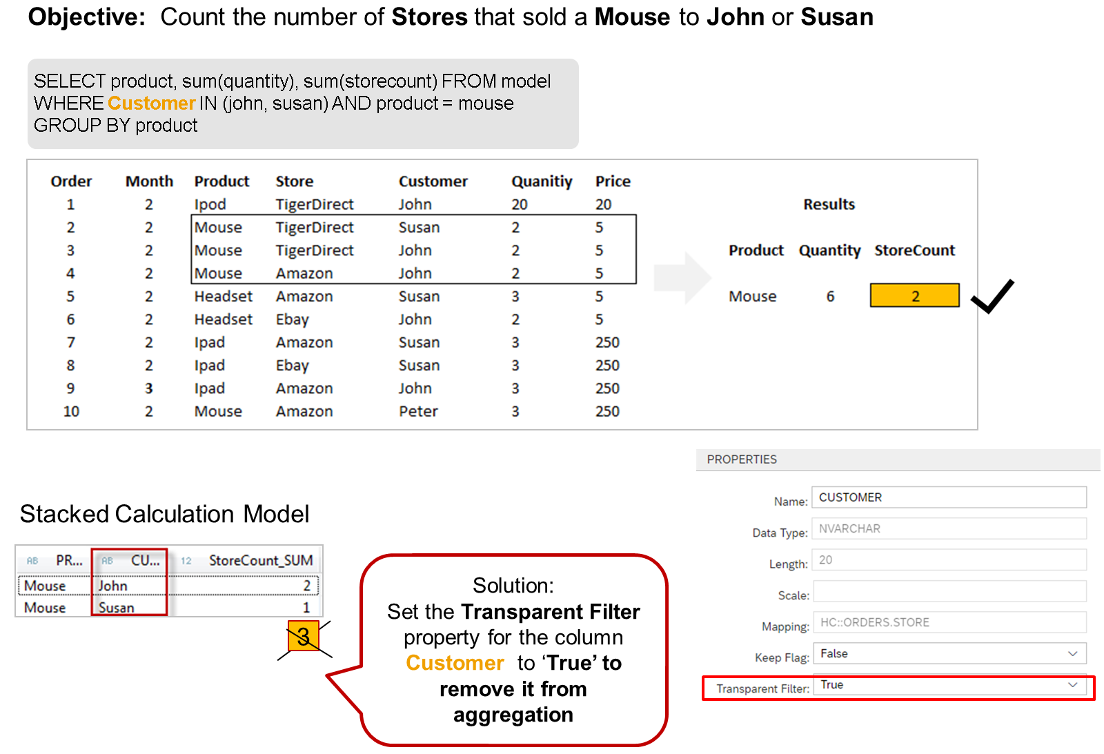
- Transparent Filter
- In this scenario, for example, calculating the number of stores that sold mice to John or Susan triggers an intermediate calculation of the StoreCount sum by product and by customer, instead of calculating the StoreCount by product.
- Setting the Transparent Filter property to true for all models and nodes that reference the Customer column will stop the Customer column from being unnecessarily used in the Group By clause.
- This property is required in the following situations:
- When using stacked views where the lower views have distinct count measures ⇒ By setting the Transparent Filter property to true, you ensure that the distinct count measures are aggregated correctly, even when filters are applied in the upper view.
- When queries executed on the upper calculation view contain filters on columns that are not projected
- If a filter defined in a lower node of a calculation view should be transparent for another view that consumes it, you must select the Transparent Filter property of all nodes from that node up to the top calculation view node.
- Rank Node
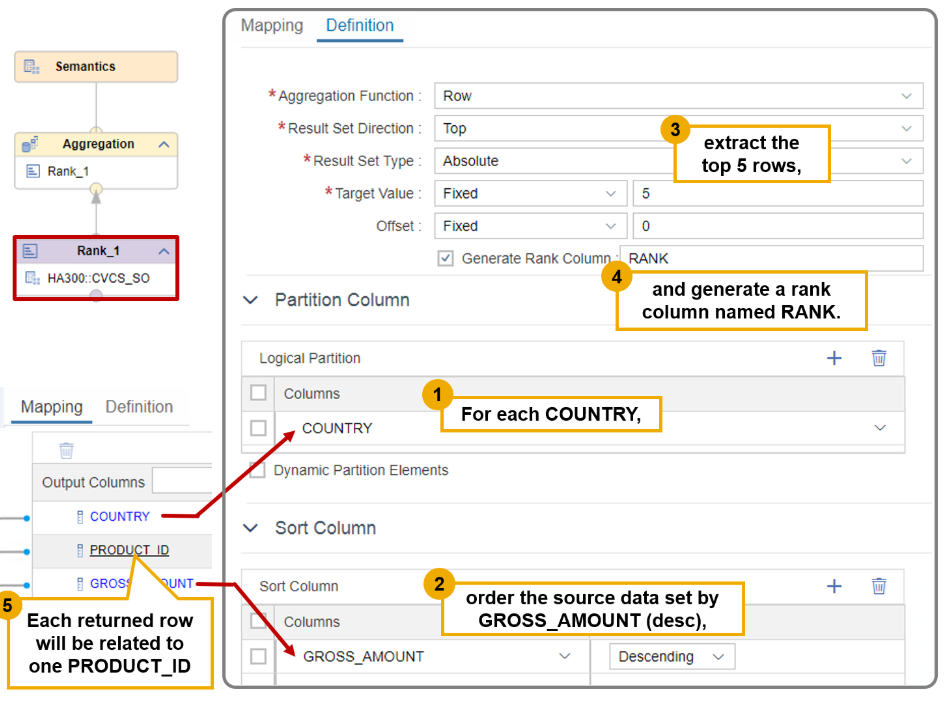
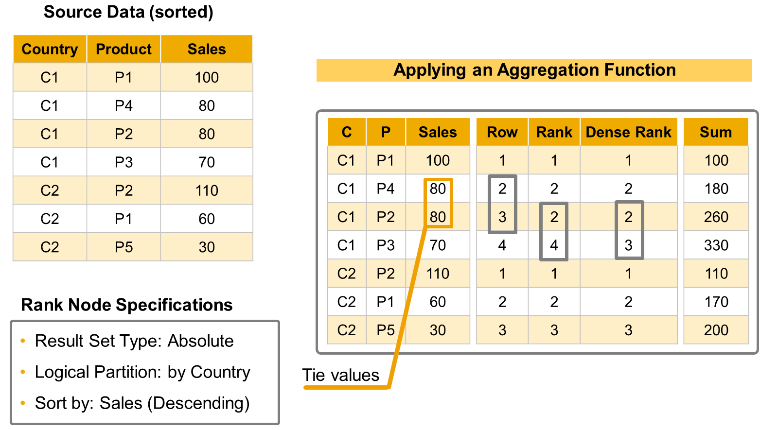
- The purpose of the Rank node is to enable the selection, within a data set, of the top or bottom 1, 2, … n values for a defined measure, and to output these measures together with the corresponding attributes and, if needed, other measures.
- For example, with a Rank node, you can easily build a subset of data that gives you the five products that generated the biggest revenue (considering the measure GROSS_AMOUNT) in each country. The country, in this example, defines a Logical Partition of the source data set.
- Rank node can partition the source data, but it does NOT perform any aggregation on the source data.
- When the source data for the Rank node is a table, you must make sure that the data structure suits your modeling needs. If not, you might need to first aggregate data by adding an Aggregation node used as a data source by the Rank node.
- When the source data for the Rank node is a CUBE calculation view, the aggregation defined in that calculation view is implicitly triggered based on the columns requested by the rank node, but a column that is mapped to the output of the Rank node but not consumed by the upper node will not be requested to the data source.
- As is the case with other types of nodes, some columns are passed to the upper nodes even when they are not requested. For example, this is the case when the calculation view has a sort order defined in the Semantics node (all the columns used for sorting are passed to consuming views). This is also the case when special settings such as Keep Flag are used.
- Aggregate Function
- Rank, row, dense rank,
- sum ⇒ The Sum aggregation function generates a cumulative sum of the sorted column up to the target value.
- Result Set Direction ⇒ Top
- Result Set Type ⇒ Absolute/Percentage
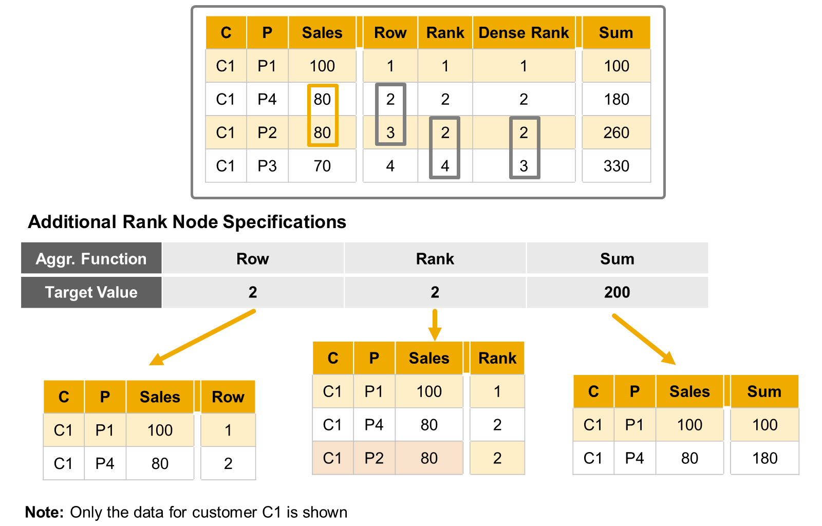
- Target Value
- Fixed or Input Parameter or All Values⇒ Top 5
- Define the number of rows to return
- The setting must be a rank value – for example, extract the data up to the rank 2), except for the Sum aggregation function where you set a cumulative value (for example, extract the data up to a cumulative Sales amount of 200).
- SAP HANA Cloud QRC 2/2024 introduces an additional capability: you can now set the Target Value setting to All Values. The rank node then sorts the value without eliminating any of them from the result set.
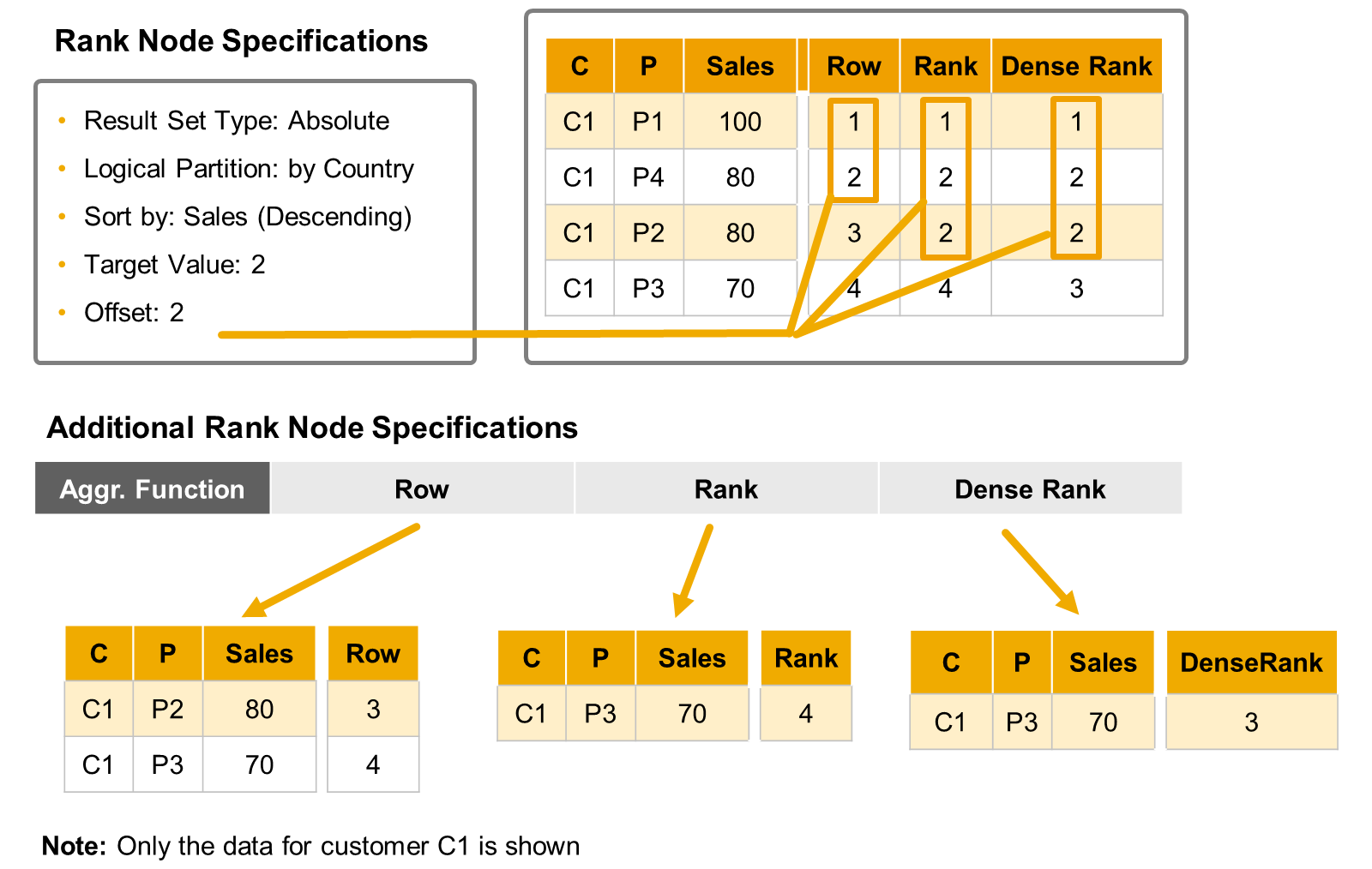
- Offset
- It is possible to exclude a number of elements from the top of the sorted data set by defining an offset.
- Generate a rank column ⇒ A new column can be generated which provides the blank position
- Partition Column
- Partition the source data set by one or several columns, before executing the rank computation
- Each row in the result will be related to an individual value or combination of values of the columns that are not included in the logical partition definition so in this case with our settings the result will display the top five products for each country based on the gross amount each row will be for one product
-
Dynamic Partition Element
- If you choose, the columns listed in the Partition will be ignored if they are not requested by an upper node or top query. To follow the same example, you could return the top five total sales for each Country only, for each year only, just by excluding the column you do not need from your top query, and without redesigning your calculation view.
- Sort Column
- Within each partition the data is sorted by one or several columns
- the aggregation functions Row, Rank, and Dense Rank will process the sort columns in the order they are listed
- This helps manage identical values in the first sort column by using the subsequent sort columns to break ties.
- The Sum aggregation function only uses the first Sort Column.
- Aggregation Node
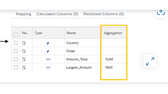
- The purpose of an Aggregation node is to apply aggregate functions to measures based on one or several attributes. The node generates a result set that is grouped by the selected attribute columns and computes the selected measure with the specified function, such as SUM, MIN, AVG, and so on.
- By default, the granularity of the aggregation is defined by the attribute columns that are mapped to the output of the aggregation node. In the example, you will get one aggregate row for each country/order pair showing two measures: the total amount of each order, and the biggest line item of each order.
- If you want to get the total amount and biggest order amount at the country level, removing the Order column from the output in semantics is not enough because you will still get the biggest line item detail in each country.
- To correctly calculate both the total amount and the largest order amount at the country level in SAP HANA Cloud, you need to use two aggregation nodes in sequence. Here's why:
- Example Data: #
- | Country | OrderID | Amount |
- |————-|————-|————|
- | US | 100 | 50 |
- | US | 100 | 30 |←Line items for Order 100
- | US | 200 | 100 |
- | UK | 300 | 20 |
- | UK | 300 | 40 |←Line items for Order 300
- Incorrect Approach (Single Aggregation Node)
- If you aggregate at the country level directly only by removing order from semantic output:
AGGREGATE BY Country MEASURES: SUM(Amount) AS TotalAmount, MAX(Amount) AS LargestOrder- Result:
- | Country | TotalAmount | LargestOrder |
- |————-|——————-|———————|
- | US | 180 | 100 |←MAX picks the largest line item (100), not the largest order total.
- | UK | 60 | 40 |←MAX picks the largest line item (40), not the largest order total.
-
Issue: The "largest order" is incorrectly calculated because it ignores the total of multi-line orders (e.g., Order 100 in the US has a total of
50 + 30 = 80
, butMAX
picks100
from Order 200). - Correct Approach (Two Aggregation Nodes)
- Step 1: Aggregate by Country and OrderID #
- First, calculate the total amount per order:
AGGREGATE BY Country, OrderID MEASURES: SUM(Amount) AS TotalPerOrder- Intermediate Result:
- | Country | OrderID | TotalPerOrder |
- |————-|————-|———————-|
- | US | 100 | 80 |←Total for Order 100
- | US | 200 | 100 |
- | UK | 300 | 60 |←Total for Order 300
- Step 2: Aggregate by Country #
- Now calculate the total amount and largest order at the country level:
-
AGGREGATE BY Country MEASURES: SUM(TotalPerOrder) AS TotalAmount, MAX(TotalPerOrder) AS LargestOrder - Final Result:
- | Country | TotalAmount | LargestOrder |
- |————-|——————-|———————|
- | US | 180 | 100 |←Correctly picks the largest order total (100 for Order 200)
- | UK | 60 | 60 |←Correctly picks the largest order total (60 for Order 300)
- Why Two Nodes Are Necessary
- 1. First Node: Groups data by
Country
andOrderID
to calculate the total for each order (TotalPerOrder
). This ensures multi-line orders are summed before comparing sizes. - 2. Second Node: Aggregates the results from the first node to compute the final
TotalAmount
(sum of all orders) andLargestOrder
(max ofTotalPerOrder
). - Without the first node,
MAX
would operate on individual line items, not the full order totals. The two-step process guarantees accuracy for both metrics. - If you exclude an attribute from an upper node (in the same calculation view or another one that consumes it), or in a query executed on top of this view, by default these attributes are ignored. In addition, the calculation view aggregates the result set on the remaining attributes.
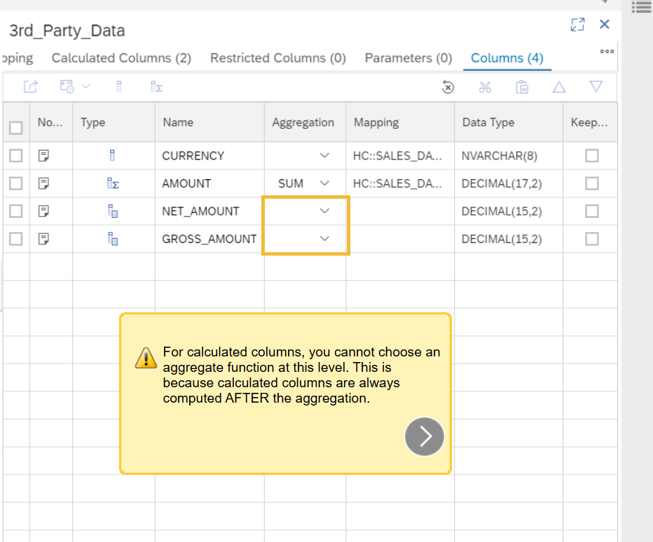
- In an Aggregation node, a calculated column is always computed AFTER the aggregate functions. If you need to calculate a column BEFORE aggregating the data from this column, you have to define the calculated column in another node, for example a Projection node, executed BEFORE the aggregation node in the calculation tree.
- Calculated columns
- Star Join node
- which is used to model a star schema, also defines one or several joins between a main data sources (fact "table") and the dimension calculation views.
- Union node
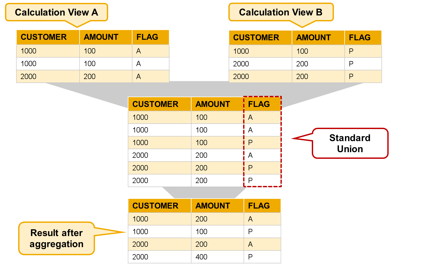
- Standard union
- A union node can be implemented in a dimension, cube and cube with star join calculation views.
- the SAP HANA Union node in calculation views is designed to work similarly to a
UNION ALL
operation. - The source column does not have to have the same name as the target column. For example, a source column month could be mapped to a target column period. Although column names can differ between the source and target (like month to period), the mapped columns must have the same or compatible data types to ensure proper unioning.
- does not have to provide a mapping for each source column. In other words, there could be source columns that are left behind and play no part in the union. This scenario is useful when you want to combine measures from multiple sources into one column. As the data sources can provide an attribute that describes the type of measure (for example, Plan or Actual),
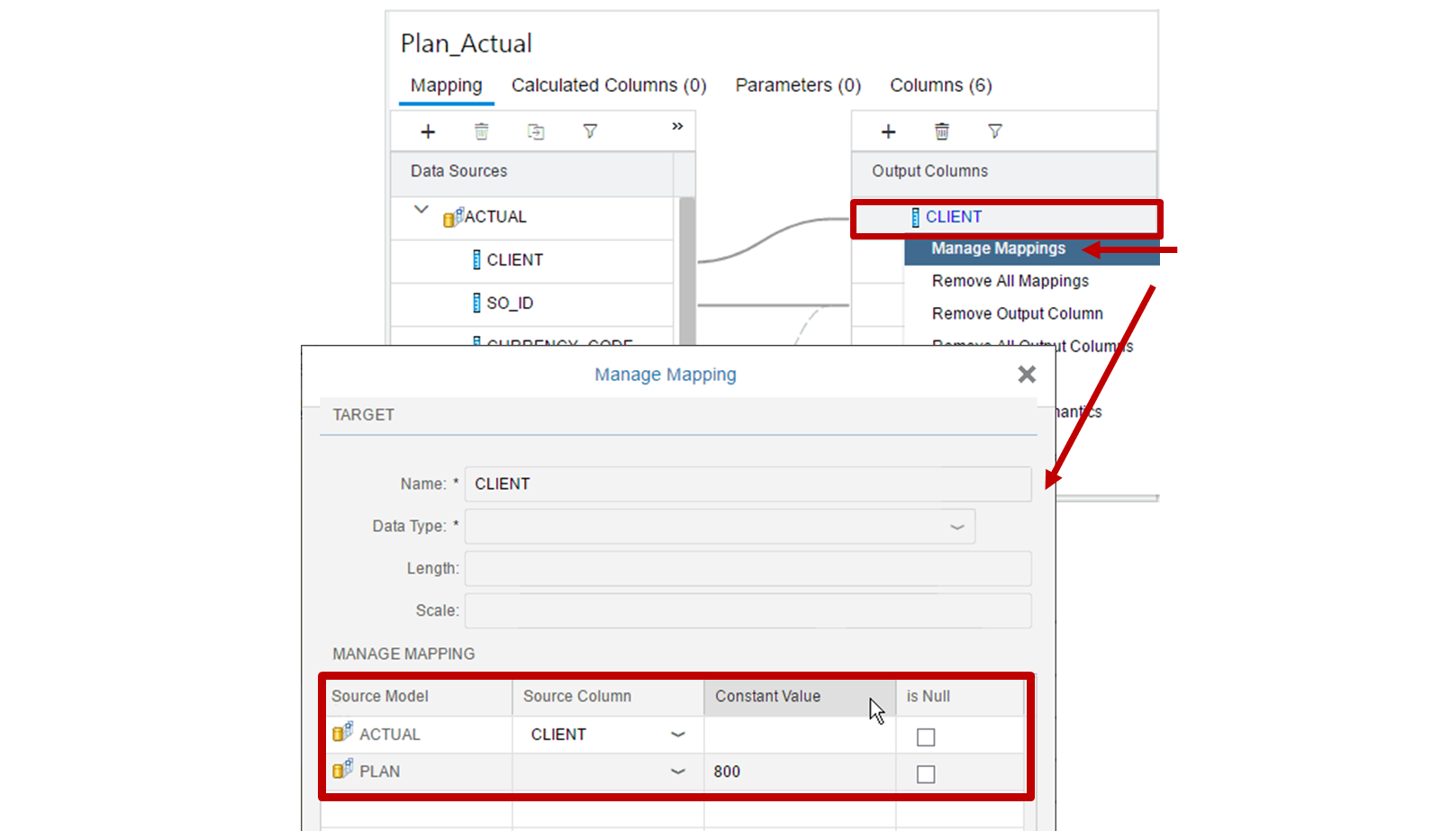
- Union with constant
- Is where you provide a fixed value that is used to fill a target column where the data source cannot provide a mapped column. For example, you have a data source that provides the actual amount and you also have a second data source that provides the planned amount. You decide to avoid combining these measures into one column as they would lose meaning, because there is no attribute to describe the meaning. In this case, you would map the measure to a separate target column and provide a constant value ‘0’ to the target column for the missing measure on each side.
- Select the union node ⇒ go to mapping ⇒ Create Two output columns ⇒ gross_value_EMEA and gross_value_AMERICA
- Right click the new columns and select manage mapping
- Provide constant value let say 0
- Now you can see gross_value_EMEA is 0 for America region similarly gross_value_AMERICA is 0 for EMEA region
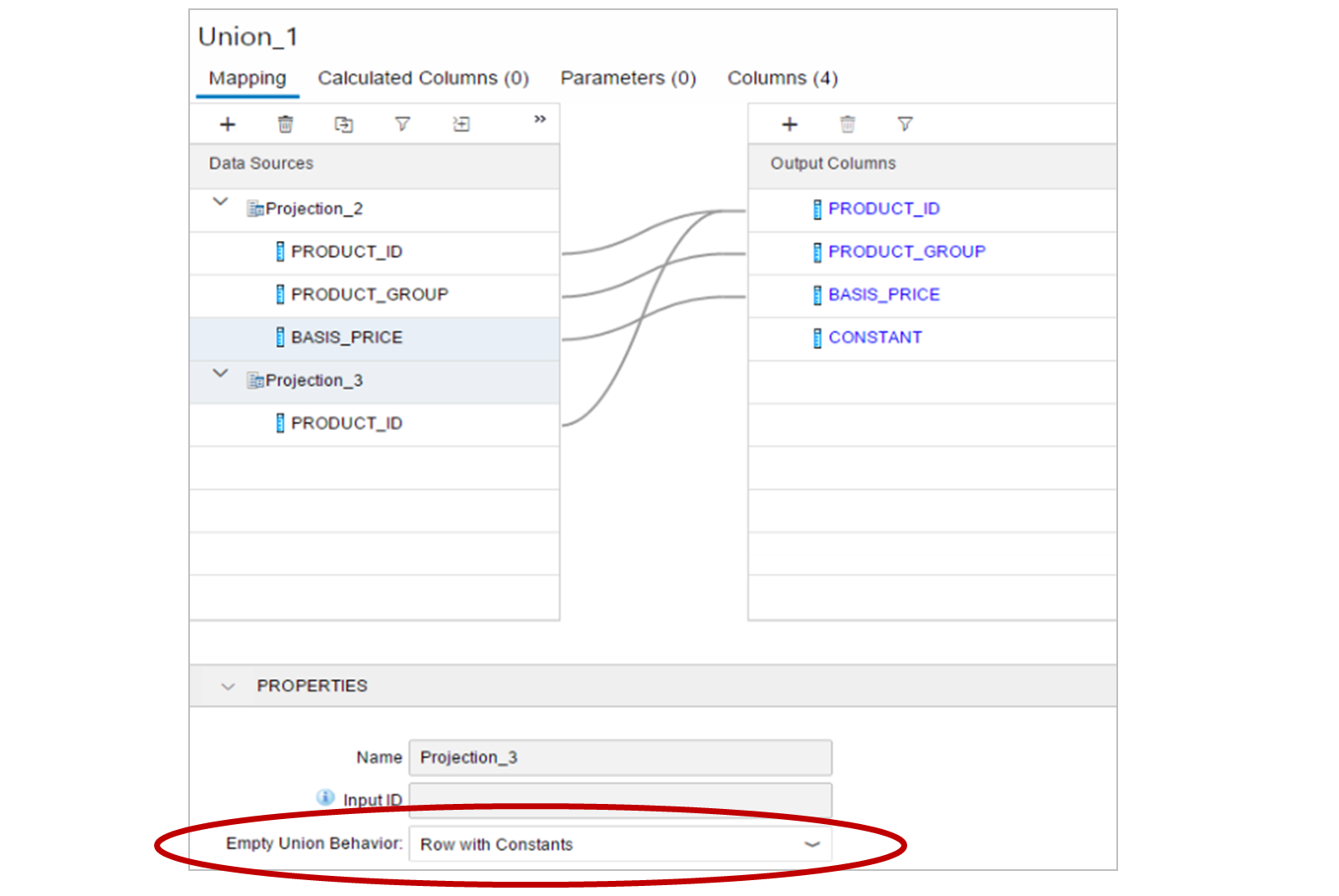
- Empty Union Behavior
- To illustrate this feature, imagine you have a data source, A, that contains the columns Product and Product Group and another data source, B, that contains only the column Product. If a query requests only the column Product Group, how does data source B respond when it does not have this column?
- The answer depends on the setting in the property, Empty Union Behavior, which is set for each data source. The default behavior, as you might expect, is to provide No Row for data source B.
- In that case, you should proceed as follows:
- Add a constant column to the union output.
- Provide a constant value for each data source with a suitable value that help you identify each source.
- Change the property Empty Union Behavior to Row with Constants.
- Define a constant value for the Product Group column for Data Source B ⇒ Union with constant
- The results will then contain multiple rows from data source A, and also a single row with the constant value that you defined for Product Group column from data source B and nulls will fill the empty columns that it could not provide.
- Union All or Union Distinct
- A Union node generates a list of all values from the input data sources, even if values are repeated. For example, if two data sources both include the same customer, then the customer will appear twice in the output data set.
- This is the equivalent of UNION ALL in SQL and is desirable in many cases.
- If repeating values are not required, you should include an Aggregation node on top of the Union node to aggregate the attributes. We normally associate aggregation Behavior with measures, such as SUM, AVE, and so on, but aggregation can also be performed on attributes. The effect of aggregating attributes is to simply produce a distinct list of values.
- This is the equivalent of UNION DISTINCT (or just UNION) in SQL.
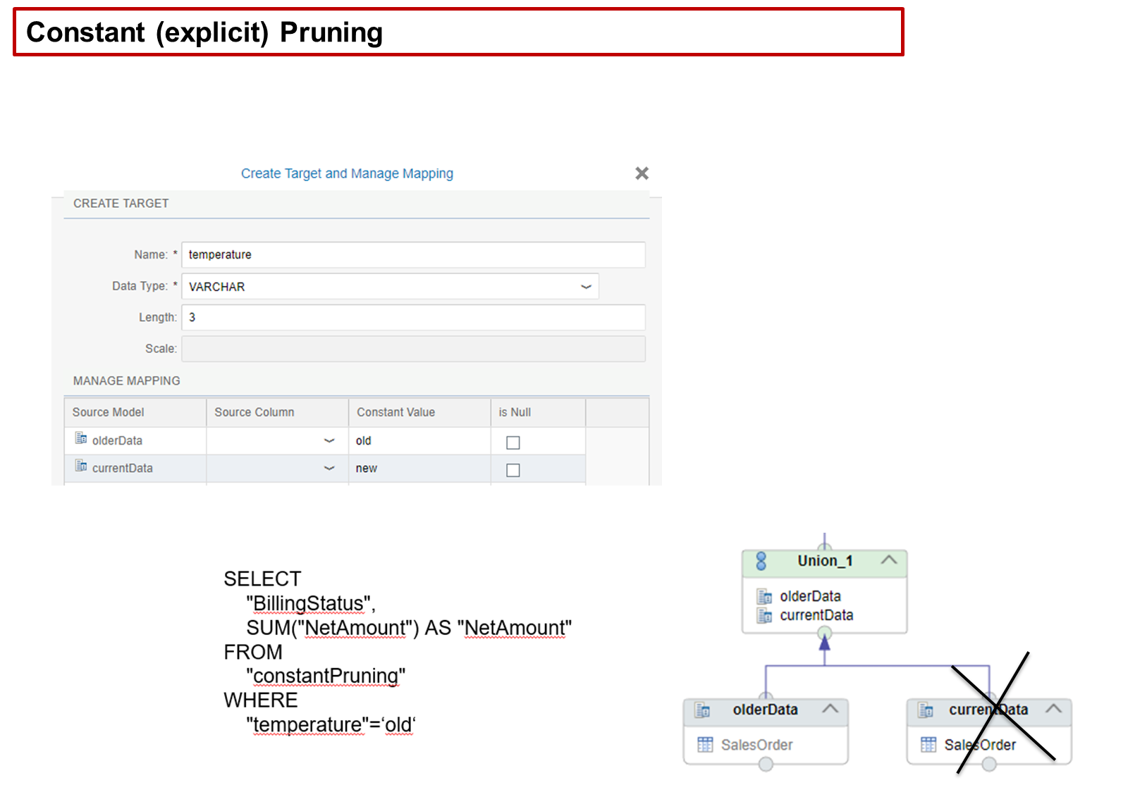
- Constant Pruning/Explicit pruning
- For each data source in a union node, you can define an additional column and fill it with a constant value to explicitly tag the meaning of the data source
- If a query filter – where clause – does not match the constant value for a specific source of a union, then the source is ignored. This is called explicit pruning. Explicit pruning helps performance by avoiding access to data sources that are not needed by the query.
- the union node has a new column defined in the union node. To assign the constant value, we use the Manage Mapping pane and enter a constant value for the new column per data source. In our case, the new column is named temperature. In our case, either the value old or new is assigned. This is a simple way to prune data sources in unions where the rules are simple and rarely change.
- Although a union node usually has just one constant column, you can create and map multiple constant columns and use AND/OR filter conditions in your query. However, a key point is that if you do not explicitly refer to the constant column in the sending query, then the data source is always included in the union and is not pruned.
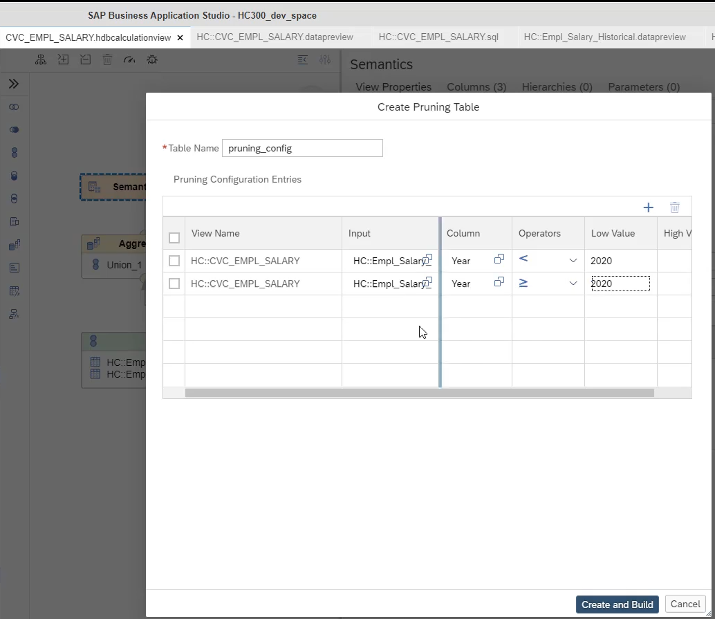
- Pruning configuration table
- configuration table sits outside the calculation view and allows you to describe in greater detail the rules that determine when each source of a union is valid.
- approach does not need to provide constant values in the union node for each data source inside the calculation view. With the table, you can define multiple single values per column that are treated with ‘OR’ logic. You can also use the greater than and less than operators. You can as well define values across different columns in a rule. Values across columns are treated with ‘AND’ logic.
- eg COUNTRY = 'US' OR COUNTRY = 'UK' AND STATE = 'NY'
- Go to Semantic ⇒ view properties ⇒ advanced ⇒ Create Pruning configuration table
- Table name
- View name ⇒ Union_prune
- Input ⇒ projection_1
- Column ⇒ COUNTRY
- Operators ⇒ equal
- Low Value ⇒ any value DE or US
- If you execute the SQL with where COUNTRY = 'DE' , Then union is pruned
- The possible operators are =, <, >, <=, >= and BETWEEN.
- If several pruning conditions exist for the same column of a view, they are combined with OR.
- On different columns, the resulting conditions are combined with AND.
- For example, you could define that a source to a union should only be accessed if the query is requesting the column YEAR = 2008 OR YEAR = 2010 OR YEAR between 2012 – 2014 AND column STATUS = ‘A’ OR STATUS = ‘X’.
- This means that if the requested data is 2008 and status ‘C’, then the source is ignored. If the request is for 2013 and status ‘A’, then the source is valid.
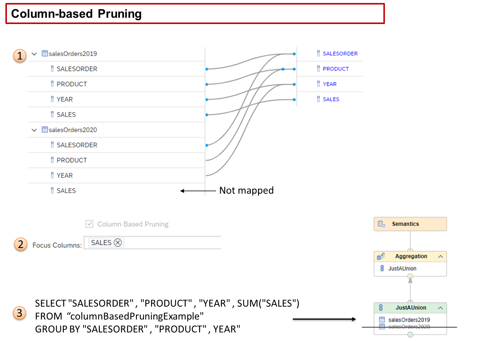
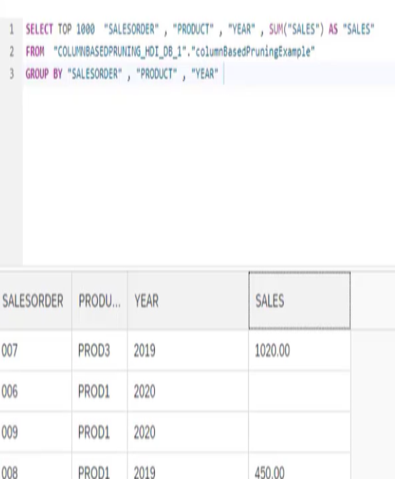
- Column-based Pruning
- Column-based pruning is another approach to eliminating data sources within unions that are not required by queries. However, unlike the other approaches, which are based on checking column values, column-based pruning looks at whether specific columns have been requested by a query and if those columns are defined as important to a result set.
- In our graphic, we see that both data sources could provide the SALES column, but only one data source salesOrder2019 provides the column to the output.
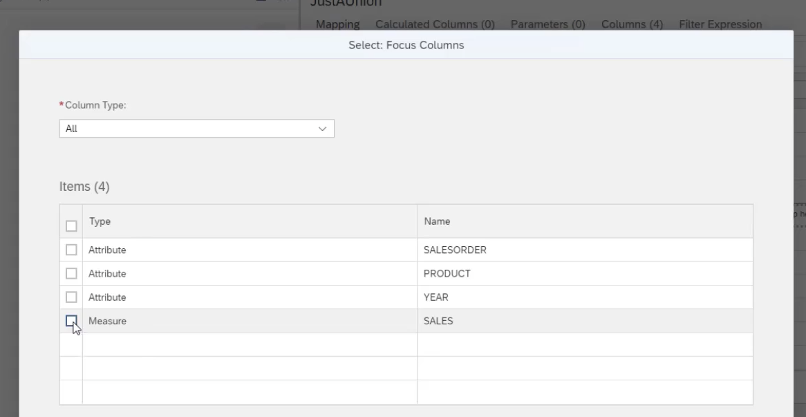
- We also see that the SALES column has been defined as a Focus Column, which means that if a query requests this column and the data source cannot provide it then we are not interested in that data source, even if other columns (YEAR and so on) could be provided.
- It is possible to define multiple Focus Columns and they can be attributes or measures or a mix of both.
- Before setting focus columns
- After setting focus column we don't see the 2020 records because even though the data source for 2020 provided Year and product data we completely neglected the data source for 2020
- Standard union
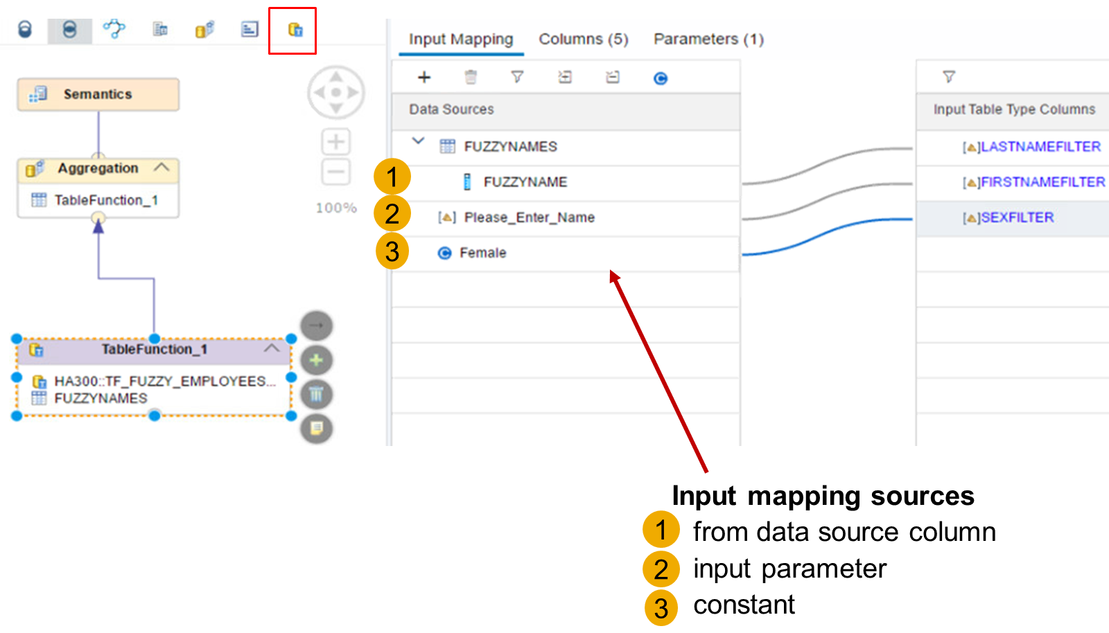
- Table Function Node
- This node is specially dedicated to the handling of the different types of mapping of the input parameters of a table function.
- There are three types of input mapping available in the Table Function node. They are as follows:
- Data Source Column
- First, add a data source to the Table Function node. Then, map one of the data source columns to one or more table function input parameters.
- Input Parameter
- Choose an input parameter from the calculation view and map it to one or more table function input parameters. This could be useful when you want a user to manually enter a value at runtime.
- Constant
- Manually define a single, fixed value, and map it to one or more table function input parameters. This is really only useful when the input value rarely/never changes.
- Window function nodes