02.Causation05.Propensity scores - sporedata/researchdesigneR GitHub Wiki

• Propensity scores are used when attempting to derive causal inferences from observational datasets, leading to a granularity of confounding control that is considered better than the one achieved through traditional regression modeling [1].
• To Compare the effectiveness of pharmacologic therapies.
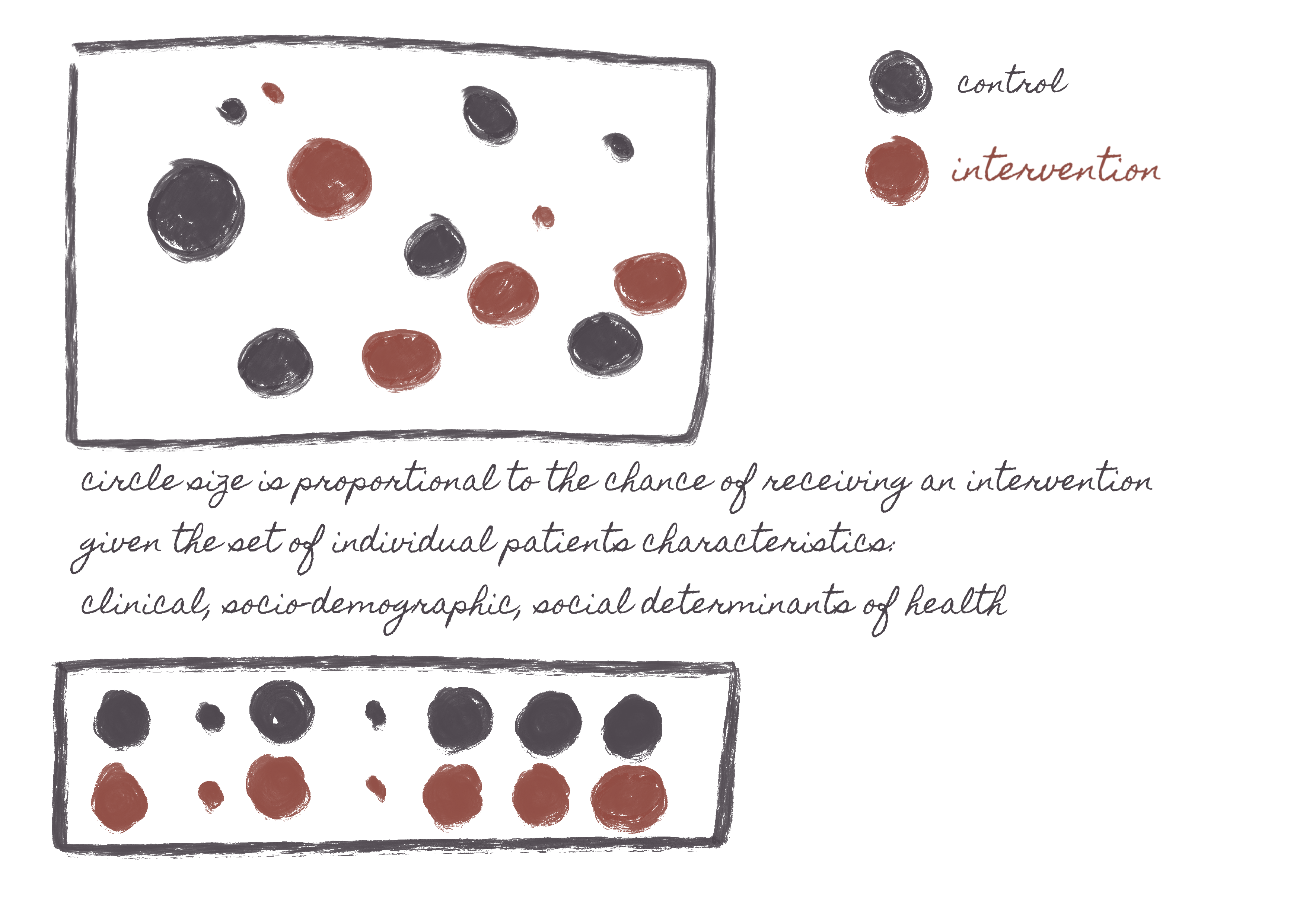
• It mimics the results of a randomized trial by forcing a balance between two or more groups receiving different interventions. It does this by predicting how likely a patient might be to get a given treatment, then you compare people who (a). have either received or not received the treatment and (b). have similar probabilities of receiving the treatment. -- (The reasoning is that if two people have similar probabilities of receiving treatment, they are similar. If they are similar, but one did receive the treatment, and the other didn't, whatever differences in outcomes they might have can be causally attributed to the treatment.)

1. Pre-requisits for causal-analysis.
2. There is a belief that the main intervention causes the outcome variable, i.e., that the introduction of the intervention will independently lead to changes in the outcome over time.

• Propensity scores only partially account for unmeasured confounding through high-dimensional propensity score adjustment [2], which means that the primary variables adjusted for inferences course are measured variables.

• The propensity score attempts to mimic a randomized controlled trial by calculating the probability of an individual receiving the treatment and then using different mechanisms to balance these individuals' distribution between or among the intervention groups. [10]. These balancing mechanisms can involve:
  • matching
  • stratification
  • inverse probability weighting
• Although the initial propensity score models were developed for dichotomous interventions, propensity score matching can also be used for:
  • multiple treatments
  • continuous treatment doses
  • within structure equation models
  • multilevel data
• Propensity scores can only adjust for measured variables, while randomized trials and other econometric methods (difference in differences, instrumental variables, regression discontinuity design) can adjust for measured and unmeasured variables. Some experiments have been conducted concerning high-dimensional propensity score adjustment [2] under the hypothesis that if one can achieve balance for a large number of measured potential confounders, then the non-measured confounders would be indirectly adjusted, but the results have been mixed [3].
• Bayesian methods for propensity score matching [4], allowing researchers to combine the advantages of multilevel Bayesian models with causal inferencing. Propensity scores and causal models, in general, are not immune to misclassification problems that are often present in secondary data [5]. Methods to address that misclassification are reported in our section on data sets.
• Doubly robust estimation combines a form of outcome regression with a model for the exposure (i.e., the propensity score) to estimate the causal effect of an exposure on an outcome. When used individually to estimate a causal effect, both the outcome regression and propensity score methods are unbiased only if the statistical model is correctly specified. The doubly robust estimator combines these two approaches, so we only need to accurately determine one of the two models to obtain an unbiased effect estimator. In other words, the doubly robust estimation combines two approaches to estimating the causal effect of an exposure (or treatment) on an outcome: (1) a regression model of the outcome and (2) weighting by the propensity score using the inverse probability weighted (IPW) approach. Thus, the effect estimator is robust to misspecification of one (but not both) of these models [13].

The following libraries are available:

• cobalt and WeightIt - These packages are associated with the automation of the balancing between the interventions. They allow trimming strategies so that extreme values of IPW do not necessarily skew the causal assessment. They also enable to choose between ATE (average treatment effect -- averaging the propensity score and then applying it to each group) and ATT (average effect treatment on the treated -- applying propensity score to each individual i.e., treatment and control) for IPW [11], [12]. ATT calculates the effect just among the group of treated patients, and the average effect treatment on the untreated (ATU) is just among the non-treated patients. ATE is for both groups if they had or had not gotten the interventions.
• DoWhy from Microsoft - DoWhy is a Microsoft-developed Python library for causal inference. It generates directed acyclic graphs (DAGs) and supports the estimation of the average causal effect logically and comprehensively by choosing from various approaches such as instrumental variables, the difference in difference, etc.

The first equation is a regression model predicting the probability of having a given intervention, having all confounders as predictors. Note that the study outcome variables are ignored in this model. The assumption is that any two people with the same probability of having an intervention have a similar distribution of their confounders. A logistic regression model is often used when there are only two types of intervention.

With the probability of having an intervention determined, we will split patients into those actually receiving and not receiving the intervention while adjusting for the probability of receiving the intervention. The second equation then compares patients with and without the intervention while adjusting for that probability: matching patients with similar probabilities (1:1 or higher) and using inverse probability weighting are among the most common models.

• Bayesian multilevel models
• Doubly robust estimation. We can use the doubly robust approach to estimate the causal effect of an exposure (or treatment) on an outcome. As an advantage, the doubly robust approach reduces bias since the effect estimator is robust to misspecification of one (but not both) of the two models (regression and IPW). Since we calculate the doubly robust estimator for the effect of exposure by averaging over the expected response for each individual under both exposure conditions, the effect estimates apply to the total population and have a marginal interpretation similar to that from a randomized trial. Besides that, the doubly robust estimator simultaneously produces relative and absolute effect estimates. The ease with which one can estimate absolute risks and risk differences can facilitate reporting of these effects along with the usual ratio measures and encourage researchers to more fully interpret their findings on both scales. The standard IPW estimator also has this advantage, but the "augmentation" that makes this estimator doubly robust makes it more efficient than the usual IPW estimator.

Nevertheless, the doubly robust estimator is less efficient than the maximum likelihood estimator with a correctly specified model. Thus, there is a trade-off between potentially reducing bias at the expense of precision. In the context of IPW estimators, weights for individuals with unusual combinations of characteristics and exposures can lead to unstable estimates with relatively large standard errors. It is unknown whether the methods for handling these influential observations (stabilized and truncated weights or trimming observations) would be effective for the doubly robust estimator or if other approaches to diagnosing and mitigating this bias are required. Moreover, when both models are misspecified, the effect estimate may be more biased than a single, misspecified maximum likelihood model.

Many aspects of applied doubly robust analysis have not yet been adequately evaluated, including strategies for selecting covariates for inclusion in the component models, diagnostics, methods for detecting and handling effect measure modification, and reconciling differences between effect estimates from doubly robust, IPW, propensity score, and maximum likelihood methods. Thus, this method should be considered a complement rather than a substitute for other methods.

1. Books

• Practical Propensity Score Methods Using R

2. Articles combining theory and scripts
   • US Food and Drug Administration Approvals of Drugs and Devices Based on Nonrandomized Clinical Trials [7].
   • The propensity score [8].
   • Using propensity score methods to create target populations in observational clinical research [9].
   • Practical guide to health policy evaluation using observational data.
   • Common references for causation.

• Characteristics of the 14-day and the 30-day mortality assessment cohorts See full table here.

• Patient characteristics for the 14-day mortality assessment cohort before and after propensity score matching. See full table here.

• Patient characteristics for the 30-day mortality assessment cohort before and after propensity score matching. See full table here.

A common concept to represent propensity scores are in silico randomized controlled trials. The reason is that propensity scores can mimic, to an extent, the results of randomized trials. The obvious exception is that non-measured variables cannot be accounted for in propensity score matching, while randomized trials account for both measured and unmeasured variables.

Reporting and Guidelines in Propensity Score Analysis

• Propensity score

• sdatools::PropensityScoreAnalysis

[1] Normand SL, Landrum MB, Guadagnoli E, Ayanian JZ, Ryan TJ, Cleary PD, McNeil BJ. Validating recommendations for coronary angiography following acute myocardial infarction in the elderly: a matched analysis using propensity scores. Journal of clinical epidemiology. 2001 Apr 1;54(4):387-98.

[2] Schneeweiss S, Rassen JA, Glynn RJ, Avorn J, Mogun H, Brookhart MA. High-dimensional propensity score adjustment in studies of treatment effects using health care claims data. Epidemiology (Cambridge, Mass.). 2009 Jul;20(4):512.

[3] Wyss R, Schneeweiss S, van der Laan M, Lendle SD, Ju C, Franklin JM. Using super learner prediction modeling to improve high-dimensional propensity score estimation. Epidemiology. 2018 Jan 1;29(1):96-106.

[4] Kaplan D, Chen J. Bayesian model averaging for propensity score analysis. Multivariate behavioral research. 2014 Nov 2;49(6):505-17.

[5] Wood M, Chrysanthopoulou S, Nordeng H, Lapane KL. The impact of nondifferential exposure misclassification on the performance of propensity scores for continuous and binary outcomes: a simulation study. Medical care. 2018 Aug;56(8):e46.

[6] Templeton AJ, Booth CM, Tannock IF. Informing Patients About Expected Outcomes: The Efficacy-Effectiveness Gap. Journal of Clinical Oncology. 2020 May 20;38(15):1651-4.

[7] Razavi M, Glasziou P, Klocksieben FA, Ioannidis JP, Chalmers I, Djulbegovic B. US Food and Drug Administration Approvals of drugs and devices based on nonrandomized clinical trials: a systematic review and meta-analysis. JAMA network open. 2019 Sep 4;2(9):e1911111-.

[8] Haukoos JS, Lewis RJ. The propensity score. Jama. 2015 Oct 20;314(15):1637-8.

[9] Thomas L, Li F, Pencina M. Using propensity score methods to create target populations in observational clinical research. Jama. 2020 Feb 4;323(5):466-7.

[10] Austin PC. [An introduction to propensity score methods for reducing the effects of confounding in observational studies.] Multivariate behavioral research. 2011 May 31;46(3):399-424.

[11] Abdia, Y., Kulasekera, K.B., Datta, S., Boakye, M. and Kong, M.Propensity scores based methods for estimating average treatment effect and average treatment effect among treated: a comparative study. Biometrical Journal, 2017.

[12] Morgan, S.L. and Winship, C Counterfactuals and causal inference. Cambridge University Press, USA; 2015.

[13] Funk, M.J., Westreich, D., Wiesen, C., Stürmer, T., Brookhart, M.A., Davidian, M. Doubly robust estimation of causal effects. American Journal of Epidemiology. 2011 Apr 1;173(7):761-767.