01.Association03.Models for outcomes measured a single time - sporedata/researchdesigneR GitHub Wiki

• These models are used when one wants to establish a non-causal association between a risk factor and an outcome, adjusted for a group of confounding variables. There are several frameworks under this category, the most well-known being GLM (generalized linear models), GAM (generalized additive models -- runs a series of small, piecewise models for different segments of a study sample), and GAMLSS (generalized additive models for location, scale, and shape). Their choice largely depends on whether the dependent variable might or not belong to the exponential family [1].

1. Cross-sectional data
2. The outcome variable is continuous, dichotomous, count, ordinal, nominal, or multivariate.

Methods fall under Nelder's Generalized Linear Model (GLM) with different types of response variables (continuous, dichotomous, count, ordinal, nominal, or multivariate), GAM (generalized additive models) and GAMLSS (generalized additive models for location, scale, and shape).

The model usually makes a few assumptions, including a linear relationship between outcomes and predictors (you can get around that, but that's a bit more advanced), normal distribution, no or little collinearity, no auto-correlation, and homoscedacity (variance is constant).

Typically, we do not use frequentist multi-level models, since they have several disadvantages, such as difficulty converging when the groups have small samples or have limited data [3].

Generalized linear models (GLM), multiple linear regression (MLR), Logistic regression (LR), Poisson, Account model (AM), Negative binomial (NB), and zero inflated models (ZIM)

Objections to automated stepwise procedures include: stepwise methods do not rely on any theory or understanding of the data; stepwise methods test hypothesis that is never asked, or even of interest or relate to multiple testing issues (standard errors of the regression parameter estimates in the final model are too low; P-values are too small; confidence intervals are too narrow; R2 values are too high; the distribution of the ANOVA test statistic does not have an F-distribution; regression parameter estimates are too large in absolute value; models selected using automated procedures often do not fit well to new data sets) [2].

These models do not account for competing risks or events (competing nature of multiple causes to the same event). As a result, they tend to produce inaccurate estimates when analyzing the marginal probability for cause-specific events. For example, while evaluating complications, a patient with severe illness undergoing ECMO therapy might die before they have a complication. This would distort the association since sicker patients would have fewer complications (because they are dead), and it introduces bias in the analysis by making it look good when it is not.

N.B.

Although some articles have stated that standard errors (and the corresponding 95% CI) should be calculated using robust methods, more reliable results can be attained with regular GLM and GEE compared with regular standard errors. Meanwhile, sandwich estimators can be used to estimate the standard errors (SE) using a variance-covariance (vcov) matrix that is not under the assumption of independently and identically distributed (IID) errors. A vcov matrix under the IID assumption implies that your data must have no serial correlation (i.e., no residuals correlation for different observations of the same individual), no cross-correlation (i.e., no residuals correlation for different individuals within or across the same period), and the same variance for the residuals (a.k.a., heteroscedasticity). These assumptions are very hard to hold for clustered data, and if you keep using regular standard error estimation, you might end up with biased errors, which will affect the p values and lead to a biased significance interpretation of the coefficient estimates.

You can use the sandwich package to generate several estimators for the robust standard error calculation for LM or GLM models in R. These estimators are provided through functions like vcovHC, which take a fitted model, extract the model matrix, and produce a vcov matrix to be used in the SE calculation. This calculation can be done with the coeftest function from the lmtest package. The same applies to GEE models, except the GEE package already provides built-in robust SEs using sandwich estimators in R.

Also,

1. Robust standard errors (which is what svy and the sandwich packages both do) are inconsistent, meaning that the corresponding 95% CI will either under or overshoot. So, we should avoid them (https://arxiv.org/pdf/2011.11874.pdf)
2. The latest approach is stacked GEE, which can be calculated using the geex package - see appendix of (https://arxiv.org/pdf/2011.11874.pdf) for code.
3. Bootstrap is the best option, as the results are accurate. However, it is not feasible in many situations since it is computer intensive (takes a long time in datasets with as many as 10k observations without even considering complex models, such as mixed-effects or cox) (https://stackoverflow.com/questions/54749641/bootstrapping-with-glm-model) and (https://socialsciences.mcmaster.ca/jfox/Books/Companion/appendices/Appendix-Bootstrapping.pdf). However, the advantage here is that you can use regular functions combined with a bootstrapping package instead of special packages.

These methods take a snapshot, capturing the association between exposure and outcome where individuals are independent from each other.

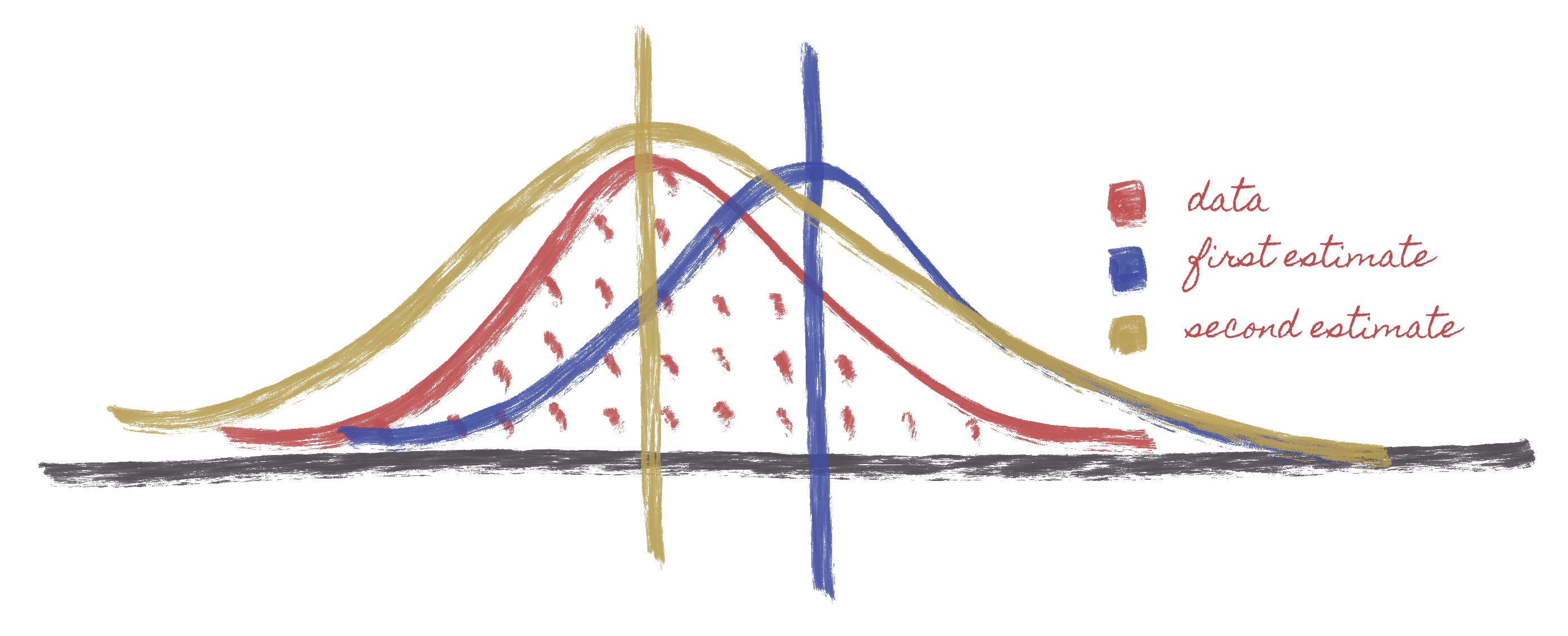
MLE takes a likelihood (a PDF or a statistical distribution) and then tells us how that distribution can be used to represent the data. The Image above describes Maximum Likelihood Estimation (MLE). This starts with the data (in red) which has a certain distribution and looks normal at first glance. You will then choose a normal distribution (Something you do when writing your code), e.g., if you are trying to model this as a GLM, you'll have to indicate wether this is a Gaussian or normal distribution, logistical distribution, poisson, etc. The algorithm will then analyze your data and throw a normal distribution with a certain mean value. For example, the first estimate that comes about (in blue) throws a normal distribution in a selected point. Nonetheless, comparing the blue and red curve, we observe a significant percentage of the area of the data outside of the normal distribution we are proposing. This initiates an optimization process - starts testing other positions for the mean, thus, allowing us to get progressively better estimates of the mean value. This further indicates that the overlap between the proposed normal distribution and the distribution of the data are getting closer until they reach a point where the is no more room for improvement. The second estimate (in gold) and the data (in red) are not the same as observed in the figure above, indicating an error between the two. The better the overlap between the mean and the red, the better the model fits. Once the mean is established, you'll then be trying to adjust the golden distribution to the red in terms of standard deviation or variants. So, you'll either squeeze, improve, or expand the curve.

Alternative methods include the use of Bayesian methods, although McElreath argues that in most cases one should use a straight [4]. Yet another alternative are Empirical Bayes Models, although Gelman is highly critical of its premises [5] and [6].

1. Generalized Linear Model (GLM)

GLM is a broad class of models that includes linear regression, logistic, and count models (Poisson, negative binomial, etc.). A generalized linear model (GLM) with a Gaussian link function is another name for multiple linear regression (MLR), thanks to their common basis [14].

In GLM, we assume that every single individual in the matrix have similar distributions, and the prediction for them is similar. Therefore there are not subgroups.

The GLM is defined for:

Where is the individual's outcome for a given individual. is a constant that represents an intercept. The intercept is the value where the line resulting from the linear regression of a dataset intersects the y axis, i.e. x = 0. The parameters to be estimated, represent the coefficients of each of the explanatory variables . Where can be metric or Dummy variables. The subscripts represent each of the sample observations under analysis (ranging from 1 to n, n being equal to the final sample size).

The is the error, which is defined as the difference between whatever this model predicts in the observation. The error is calculated using

Where, the error is Normal Identically Distributed () and represent the standard deviation fixed.

• It is important to determine the statistical distribution of response variables before estimating any confirmatory model. This will help to estimate the most appropriate parameters for predictive effects.[6]

2. Normal distribution a.k.a Gaussian Distribution.

.

As we can see, f is a function of the variable x and two parameters, mu (the population mean) and sig^2 (the population variance). To make it simpler to understand, let's set mu = 0 and sig^2 = 1. Now we have the function f(x) = K e ^ -(x^2)/2, where K is just a positive constant = 1/sqrt(2*Pi). It resembles a negative exponential function, except by the x^2 factor, which is responsible for giving the curve a symmetric bell shape. In the original function, since x is accompanied by mu in a negative/additive form, mu is responsible for sliding the curve horizontally along the x axis. On the other hand, since x is accompanied by sig^2 in a divisible/multiplicative form, sig^2 is responsible for scaling the curve vertically along the y axis. That way, the curve will be always centered by the population mean (mu) and flattened or stretched out by the population variance (sig^2). I've created a visualization where you can play with these parameters and see how they interfere in the curve's shape: here. On the "computational sense" of a function, we would call (execute) the function with these two parameters and the function will work to create the distribution based on those properties.

Importance of probability density functions (PDFs)

1. The goal of a statistical model is to find an "equation" that fits the data, so that you can describe it to either evaluate causality or make predictions [13].
2. Maximum likelihood estimation is one of the ways to find these equations, and it works by first having the data scientist subjectively choosing a distribution that matches the outcome variable, for example the normal distribution family (it's a family because the nromal curve can become a family of curves by changing two parameters).
3. Then you use something like maximum likelihood estimation (MLE) or other methods to find the best normal distribution (from the family of distributions) to your data. The "best normal distribution" means that MLE will play with different parameters from a normal distribution to make it similar to your data. Check this video
4. in the specific example of a normal distribution, there are only two parameters that MLE can play with to make it similar to your data: mean and standard deviation. How do we know that: it comes from the PDF described above.

In sum, by understanding the equation (the PDF) for the normal distribution -- and specifically how the mean and standard deviation are controlled in that normal "equation" -- you learn how to play with the normal distribution family so that you can ensure that it will match your data as well as possible

• Causal models if the goal is to demonstrate that GLM is associated with residual bias.

• Multilevel packages, with McElreath making a point that [multilevel models should be the default in most situations where today we use generalized linear models this is a very strong argument [4]. When evaluating multilevel models, you can use regression diagnostics to test the model's assumptions, which are the same as the ones we used for GLM but evaluated differently.

Regression diagnosis is a way to analyze a model's performance over the fitted data. It is critical when building a regression because it enables you to understand how well your model fits the data. In essence, it comes down to observed vs. predicted, the idea being that if the relationship between the two is not homogeneous (or has deviations), then some model assumption was probably violated (normality, homoscedasticity, collinearity, etc.). If you have any idea of the violation, you can implement a potential solution, like removing collinear variables, using variable transformation, etc. For instance:

1. Linearity is assessed through plots of residuals (observed vs. expected). Although you can get p values to help you decide, the assessment is primarily visual. If the assumption is met, the plot should look random and not display any trends.

2. Homoscedasticity or homogeneity in the variance assessed within each group through an ANOVA comparing observed and expected values. A non-significant value. Note that the definition of what a group is will depend on which groups you used for your multilevel model

3. Residuals are normally distributed, which can be visually tested using QQ plots (deviations from normality will be shown as the diagonal line moves away from the diagonal).

As with other regression diagnostics, if there is a violation, the first attempt would be to start transforming and see if they would resolve the issue. It might be worth checking here.

• Specification curve analysis; this method allows can check where a wide range of assumptions (about variable definitions, usually) will affect the final conclusions of an analysis.

1. Books

   • Generalized Additive Models: An Introduction with R
   • Semiparametric Regression with R
   • Distributions for Modeling Location, Scale, and Shape Using GAMLSS in R

2. Articles combining theory and scripts

   • GAM
   • GAMLSS
   • Odds ratios—current best practice and use
   • Marginal effects—quantifying the effect of changes in risk factors in logistic regression models
   • Generalized Linear Models

• The main risk factors for a given outcome are [LIST OF RISK FACTORS]

The odds ratio (OR) helps identify how likely a specific event (outcome) is associated to an exposure (intervention) when compared with the same event occurring in the absence of that exposure. The larger the OR, the higher odds that the event will occur with exposure. When OR < 1, it implies the event has fewer odds of happening with the exposure, whereas OR = 1 implies the exposure does not affect the odds of the event. The OR value can be reported as follows:

Compared to [referent], [intervention] presented [OR, (95% CI)] times the odds [p value] of [outcome].

The 95% confidence interval (CI) gives an expected range for the population odds ratio to fall within. It can be used to estimate the precision of the OR, where a large CI indicates a low level of precision of the OR, whereas a small CI indicates a higher precision of the OR. The CI is also used as a indicator of statistical significance for the OR if it does not overlap the null value (OR = 1). Of importance, negative CI values are just an artifact of the binomial distribution used to calculate them when the lower boundary is close to zero [7]. We can keep them as is or replace them with a zero value.

The p-value is the probability of observing the given effect at least as extreme as the one observed in the sample data, assuming the truth of null hypothesis. A p-value less than 0.05 means that observing such an extreme result under the null hypothesis would be very unlikely (less than 5% of the time), providing statistical significance to reject the null hypothesis (OR = 1).

Calculation of risk requires the use of “people at risk” as the denominator. In retrospective (case-control) studies, where the total number of exposed people is not available, risk ratio (RR) cannot be calculated and OR is used as a measure of the strength of association between exposure and outcome. By contrast, in prospective studies (cohort studies), where the number at risk (number exposed) is available, either RR or OR can be calculated [9].

Multiple logistic regression, a frequently used multivariate technique, calculates adjusted ORs and not RRs.

1. Which individuals are independents from the others.
2. Causal inferences (adjustments for potential confounders).

The main guidelines are:

• STROBE.
• RECORD-PE - The reporting of studies conducted using observational routinely collected health data statements for pharmacoepidemiology (RECORD-PE)

• sdatools::boxPlot
• sdatools::scatterPlot
• sdatools::barPlot
• sdatools::stackedBarPlot
• sdatools::likertPlot

There are literally dozens of packages involving GLM, but the base frequentist package is glm [8]. For Bayesian models, options are:

• rstan [10].
• rstanarm [11].
• brms [12].

[1] wikipedia.org. 2020. Exponential Family.

[2] Peter K. D, and Gordon KS Generalized Linear Models With Examples in R (Springer Texts in Statistics); Section 2.12.3 Objections to Using Stepwise Procedures. Springer, 2018.

[3] Detry MA, Ma Y. Analyzing repeated measurements using mixed models. Jama. 2016 Jan 26;315(4):407-8.

[4] Koster J, McElreath R. Multinomial analysis of behavior: statistical methods. Behavioral ecology and sociobiology. 2017 Sep 1;71(9):138.

[5] Halim, A., 2016. Statistical Modeling, Causal Inference, And Social Science. [online]

[6] Gelman A. Objections to Bayesian statistics. Bayesian Analysis. 2008;3(3):445-9.

[7] Brown LD, Cai TT, Dasgupta A. Interval Estimation for a Binomial Proportion. Statistical Science. 1999;16:101-133.

[8] rdocumentation.org. n.d. Glm. [online].

[9] Ranganathan, Priya, Rakesh Aggarwal, and C. S. Pramesh. "Common pitfalls in statistical analysis: Odds versus risk." Perspectives in clinical research 6.4 (2015): 222.

[10] Team SD. RStan: the R interface to Stan. R package version. 2016;2(1).

[11] Goodrich B, Gabry J, Ali I, Brilleman S. rstanarm: Bayesian applied regression modeling via Stan. R package version 2.17. 4.

[12] Bürkner PC. Brms: Bayesian regression models using Stan (R package version 1.6. 1).

[13] Madore JD. 2022. The Difference Between Functions & Equations (3 Key Ideas).

[14] Nelder JA, Wedderburn RW. Generalized linear models. Journal of the Royal Statistical Society: Series A (General). 1972 May;135(3):370-84.