Pre Day Carrier Operations Planning - smart-fm/simmobility-prod GitHub Wiki
Inputs and Data sources
| Table | Schema | Database |
|---|---|---|
| vehicles | synthpop12 | hpc |
| vehicle ownership | synthpop12 | hpc |
| establishment | synthpop12 | hpc |
| shipments | demand | hpc |
| traveltime | freight | hpc |
**Inputs and Data sources
| Procedures | Schema.Table | Database |
|---|---|---|
| get_freight_annual_contract_size | freight.contract | hpc |
| get_freight_vehicle_estbid_industry | synpop12.vehicle, synpop12.vehicle_ownership, Synpop12.establishment | hpc |
| get_freight_establishment_fleetSize | synpop12.vehicle, Synpop12.vehicle_ownership | hpc |
| get_freight_establishment | freight.establishment | hpc |
| get_freight_establishments_node_mapping | freight.establishment, Demand.postcode_node_map | hpc |
| get_freight_establishments_coordinates | synpop12.sla_addresses, freight.establishment | hpc |
| get_freight_shipments_on_curr_day | demand.shipments | hpc |
| get_freight_all_travel_times | freight.traveltime | hpc |
| get_freight_departure_time_prob | freight.DepartureTimeProbabilities | hpc |
| get_parking_access | supply.parkingaccess | hpc |
| get_node_taz_mapping | demand.node_taz_map_onetoone | hpc |
Additional inputs include:
- Firm Synthesis model, for the establishments to be considered below.
- Fleet Synthesis model, for vehicles owned by each establishment.
- Day selection model, for the table of selected shipments with details of commodity type and quantity requiring transportation between each shipper and receiver on the "simulation day."
- Establishment to network node membership
- Travel times and distance between nodes.
Methodology
The methodology of carrier selection and carrier operations planning models are connected with each model calling the other depending on need. Carrier selection assumes two types of profiles for establishments. Shippers might change from the first to the second profile but never the other way around.
-
Shipper is a carrier. Shipper-carriers are those establishments that own freight vehicles which they can use to move their goods. Shipper-carriers assign as many shipments as possible to the owned fleet of vehicles. In case of all shipments being assigned to owned vehicles, we assume that vehicles are not available for use by other shippers unless the shipper belongs to one of the industry classes in the table below.
-
Shipper must outsource transportation (to a for-hire carrier). This profile applies when the shipper has no more owned-vehicle capacity to move their goods or owns no vehicles at all. In this case, the shipper needs to select a carrier with a suitable vehicle to transport their shipments (i.e., enough capacity for the shipments being considered as well as time-availability and, if already loaded with goods, carrying goods of compatible type):
- For the Singapore application, permissible carriers are assumed as those belonging to the following industries:
| SSIC | Industry |
|---|---|
| 25 | Transportation and Storage- Land Transport |
| 26 | Transportation and Storage- Water Transport |
| 27 | Transportation and Storage- Air Transport |
| 28 | Transportation and Storage- Warehousing & Storage |
| 29 | Transportation and Storage- Post & Courier |
| 30 | Transportation and Storage- Others |
Compatibility of goods is currently assumed as being in the same goods "group" defined in the long-term models. As these "groups" are quite broad no mix is allowed. Currently other shipment characteristics - or special needs - such as need to refrigeration, etc. are ignored.
The carrier operations planning module consists in core routine and a set of subroutines which are called at several stages of the process. The subroutines are the following:
- Vehicle selection: selecting a vehicle to be assigned one or more shipments.
- Clustering heuristic: search routine to cluster shipments, destination-wise, into a vehicle. Only applicable to shippers with own vehicles.
- Routing model: calculates vehicle routes to load and unload the shipments, thus contributing to assess tour duration and also vehicle availability.
- Update vehicle availability: allows for more than one round of deliveries using vehicles with available "driving" time.
The core routine consists in the steps below, currently named "LTL" for legacy reasons. Steps 1 and 2 are usually referred to as "own-account" and steps 3 and beyond as "for-hire".
- List "Shipper-carriers" (i.e. shippers who own freight vehicles). We will iterate over this list and, for each shipper-carrier, we will iterate over their list of shipments up to when at least one of the following criteria are met: (A) There are no more vehicles to receive shipments (assumed equal to not having any vehicle with availability > than 2 hours OR (B) There are no more shipments to be shipped.
- For every "Shipper-carrier", assign shipments to owned goods vehicles using the following sequence of sub-routines:
- Select shipment furthest away from shipper as "seed"
- If this is a "direct shipment"
- Vehicle selection
- Draw stop duration for pickup and delivery (see More info / Stop duration distribution heading)
- Routing model
- Update vehicle availability
- If this is an "indirect shipment"
- Vehicle selection
- Draw stop duration for pickup and delivery (see More info / Stop duration distribution heading)
- Clustering heuristic
- Routing model
- Update vehicle availability
- If this is a "direct shipment"
- Select shipment furthest away from shipper as "seed"
- Create a list of shipments from Non-"Shipper-carriers" and shipments that remained unloaded from "Shipper-carriers".
- Create set of "Carriers" who can provide freight movement services.
- Iterate over this list of shipments for specified number of times (now set to 3) as follows:
- Select shipment
- If this is a "direct shipment"
- Vehicle selection
- Draw stop duration for pickup and delivery (see More info / Stop duration distribution heading)
- Routing model
- Update vehicle availability
- If this is an "indirect shipment"
- Vehicle selection
- Draw stop duration for pickup and delivery (see More info / Stop duration distribution heading)
- Try to assign as much remaining shipments from the same shipper that can be loaded into the vehicle (considering commodity type and capacity limits).
- Routing model
- Update vehicle availability
- If this is a "direct shipment"
- In case the vehicle availability is exceeded the vehicle/receiver pair is dropped blacklisted. There is a possibility that it can be paired with other carrier in subsequent iterations over unassigned shipments list. Once shipment(s) is/are dropped the "Update vehicle availability" module is triggered again.
- Select shipment
The modules mentioned above are described below with more detail.
Vehicle selection
The procedure starts by only considering vehicles with time availability (i.e. > min. availability) and
- Own Carrier & Direct Shipment: assign any vehicle from smallest fit vehicle type (LGV/HGV/VHGV) among own vehicles.
- Own Carrier & Indirect Shipment: assign any vehicle from smallest fit vehicle type (LGV/HGV/VHGV) among own vehicles.
- For-hire Carrier & Direct Shipment: find nearest for-hire carrier and assign any vehicle from smallest fit vehicle type (LGV/HGV/VHGV).
- For-hire Carrier & Indirect Shipments: find nearest for-hire carrier and assign any vehicle from smallest fit vehicle type (LGV/HGV/VHGV).
Note the following:
- If the vehicle has not been assigned any tour yet, then assign the vehicle a departure time from a probability distribution. More details under the More info / Departure time probability distribution heading.
- The vehicle list for each business is unordered, thus no sorting is performed, assuming that the predominant vehicle types are more likely to be selected.
- All vehicles are initialized with 12 hours maximum available time.
Clustering heuristic
- Set up the vehicle for loading:
- Set up loading limit in capacity by multiplying the vehicle capacity by a payload limit factor, thus restricting its original capacity. This constraint aims to replicate the effect of several factors we don't take into account (e.g. delivery time windows, urgent deliveries, etc.). More details on the probability distributions under the More info / Payload limit factor heading. Although the code for this constraint is available in the model it's use is not advised by Prof. Moshe-Ben Akiva due to the lack of behavioral foundation. Since it contributes to better alignment with traffic counts it's only in place up to when a better heuristic formulation replaces it. This setting can be turned off in the MT .xml file.
- Set up Number of deliveries per tour limit = number of establishments to which shipments are delivered. More details on the probability distributions under the More info / Stops per tour heading. This setting can be turned off in the MT .xml file.
- Load shipments. The method is in the sub-bullets, shipments are only loaded up to when any constraint in (3) is met.
- The initial centroid of the cluster is the coordinates of receiver of the seed shipment.
- Select the closest shipment to centroid which doesn't violate vehicle capacity nor shipment type compatibility. In case of a tie between shipments, choose any of the two shipments randomly. If shipment is successfully loaded calculate the new centroid between shipments. Iterate up to when constraints are met. Stop duration is added by receiver (establishment) using the stop duration distribution (see the heading More info / Stop duration distribution).Once constraints are met following steps ensue.
- Re-calculate vehicle capacity usage and total stops per tour
- Re-calculate tour duration (travel + stops) using "Routing Model" module.
- Trigger "Update vehicle availability".
- Constraints
- there are no more shipments to add in the cluster or for the shipper.
- there are no shipments which can be added without exceeding vehicle capacity. Note that there are various possible interpretations of capacity as detailed under the More info / Vehicle capacity settings heading.
- 'allowed' stops per tour are met.
- 'allowed' vehicle availability is exceeded.
- In case the vehicle availability is met, random shipments are selected to be dropped up to when the tour duration is not in excess of its availability. Once shipment(s) is/are dropped the "Update vehicle availability" module is triggered again.
Routing model
Note: The vehicle first leg is defined from the overnight parking location to the pickup point. Upon return of a tour it is assumed that the vehicle returns to the overnight parking location skipping the location where vehicle was loaded. In the present implementation overnight parking location is at the owners' establishment, thus the vehicle returns to the pickup location.
Route choice is performed as follows:
- A carrier is assigned
distance ortime-based routingfrom the due variable in "freight_calibration.csv".(CARRIER_SAVING_TYPE_DISTANCE_PROBABILITY variable not used at the moment.) - Node to node path sets are created for all shipments that need to be delivered from the pickup onwards.
- A number is drawn from 1 to 10. This total of pathsets are extracted for smaller travel times or distances.
- Travel time or distance is averaged across this selection of paths. Default travel time for paths is based on an LTA dataset. Travel time source is unknown but expected to be based on link free flow, i.e. equal to segment speed. Travel times are not read from the traveltime table in the freight schema.
- The vehicle iterates through the shipments in a greedy approach, selecting the closest at every new trip.
Update vehicle availability
Once triggered this routine updates the vehicle "available time" based on the "maximum usage time" and assigned tour durations.
Outputs
| Table | Schema | Database |
|---|---|---|
| fas | demand | hpc |
Also, check: Simulation Output (Freight specific)
More info
Departure time probability distribution
Note that the latest departure time is currently capped at 9:30 pm / 10:00 pm to ensure vehicles can complete the simulation. These were estimated from Tokyo data.
| time (30 min period) | share | comul share |
|---|---|---|
| 1 (00:00 to 00:30) | 0.010831447 | 0.010831447 |
| 2 | 0.014761111 | 0.025592558 |
| 3 | 0.018690775 | 0.044283333 |
| 4 | 0.022620439 | 0.066903772 |
| 5 | 0.023689905 | 0.090593677 |
| 6 | 0.02667446 | 0.117268137 |
| 7 | 0.02784341 | 0.145111547 |
| 8 | 0.032805233 | 0.17791678 |
| 9 | 0.03418559 | 0.21210237 |
| 10 | 0.040813789 | 0.252916159 |
| 11 | 0.043375532 | 0.296291691 |
| 12 | 0.048685552 | 0.344977243 |
| 13 | 0.048884523 | 0.393861766 |
| 14 | 0.042641829 | 0.436503595 |
| 15 | 0.038936006 | 0.475439601 |
| 16 | 0.035565946 | 0.511005547 |
| 17 | 0.031462183 | 0.54246773 |
| 18 | 0.023615291 | 0.566083021 |
| 19 | 0.020593429 | 0.58667645 |
| 20 | 0.018541547 | 0.605217997 |
| 21 | 0.015954933 | 0.62117293 |
| 22 | 0.016390181 | 0.637563111 |
| 23 | 0.018989231 | 0.656552342 |
| 24 (12:00) | 0.020506379 | 0.677058721 |
| 25 | 0.020767528 | 0.697826249 |
| 26 | 0.022844281 | 0.72067053 |
| 27 | 0.025032954 | 0.745703484 |
| 28 | 0.022172756 | 0.76787624 |
| 29 | 0.020195488 | 0.788071728 |
| 30 | 0.019051409 | 0.807123137 |
| 31 | 0.019275251 | 0.826398388 |
| 32 | 0.018081429 | 0.844479817 |
| 33 | 0.017397468 | 0.861877285 |
| 34 | 0.015544557 | 0.877421842 |
| 35 | 0.013828438 | 0.89125028 |
| 36 | 0.013007685 | 0.904257965 |
| 37 | 0.011378616 | 0.915636581 |
| 38 | 0.010147487 | 0.925784068 |
| 39 | 0.007734972 | 0.93351904 |
| 40 | 0.007274853 | 0.940793893 |
| 41 | 0.007075882 | 0.947869775 |
| 42 | 0.007822021 | 0.955691796 |
| 43 | 0.008953665 | 0.964645461 |
| 44 | 0.007461387 | 0.972106848 |
| 45 | 0.007075882 | 0.97918273 |
| 46 | 0.00693909 | 0.98612182 |
| 47 | 0.006976397 | 0.993098217 |
| 48 (11:30 to 00:00) | 0.006901783 | 1 |
Payload limit factor distribution
The Payload limit factor distribution was estimated using the U.S. 2002 Vehicle Inventory and Use Survey (V.I.U.S.) data, and splitting the sample of the vehicles by SG Maximum Laden Weight ranges (LGV, HVG, VHGV). We draw the payload limit per the vehicle type, between 0.1 and 1 in intervals of 0.1, from probability distributions defined by the following functions (x = limited capacity; f(x) = probability):
- LGV: f(x) = a* sin(b * x + c); a=0.173, b=3.439, c=-0.1458
- HGV: f(x) = a * exp(b * x) + c * exp(d * x); a=0.00459, b=4.803, c=-3.787e-17, d=37.02
- VHGV: f(x) = a * exp(-((x - b) / c )^2); a=0.5166, b=0.9403 , c=0.1138
Stops per tour distribution
The Stops per tour distribution was estimated using from a cumulative probability plot found in the following reference: Olszewski, P., Wong, Y. and J. Luk. 2003. FREIGHT TRANSPORT IN SINGAPORE – CURRENT STATUS AND FUTURE RESEARCH. Proceedings of the 21st ARRB and 11th REAAA Conference: “Transport: Our Highway to a Sustainable Future”. Draw an integer from the following probability distributions (x = number of deliveries; f(x) = probability):
- LGV: f(x) = a * x^b; a= 0.03694, b=-0.2351
- HGV: f(x) = a * b * x^(b-1) * exp(-a * x^b); a=0.03785, b=1.303
- VHGV: f(x)= a * b * x^(b-1) * exp(-a * x^b); a=0.007684, b=2.149
Stop duration distribution
The stop duration distribution is a log-normal distribution with mu=2.62, sigma=1.00. Note the size and quantity of the shipments is not related to the stop duration at all. The stop duration probability distribution was calculated using data from 2 datasets:LGV and HGV vehicles parked in or out loading/unloading bays for Lisbon (E.U. Project “STRAIGHTSOL”, Lisbon on-street parking observations) and Singapore deliveries to malls (Northpoint and Tampines malls including on-street parking). Its random output is limited in the code to durations between 4 and 53 minutes. While the first factor (vehicle type) was shown to be negligible, the parking location influences stop duration. Still, it is not considered now as parking selection is not yet explicitly modeled.
Number of helpers
A number_helpers attribute is added for purposes of parking choice. The presence/absence of driver’s helpers in performing the designated activity is an important attribute that influences several aspects of the parking choice behaviour:
- Given a volume of goods to be handled and a commodity type, larger the number of helpers, lower is the expected parking duration, as faster is the delivery/pick-up;
- If one or more helpers is present the driver is more risk taking in parking illegally: while the helper(s) perform the delivery/pick-up the driver can guard the vehicle and watch for patrolling traffic police car.
Attribute “number of helpers” takes integer value 1-3 at the beginning of the tour by drawing a random number from a uniform distribution and compare the value with the given probabilities described in the following table.
| Workers | 1 | 2 | 3 |
|---|---|---|---|
| LGV | 0.48 | 0.46 | 0.06 |
| HGV & VHGV | 0.75 | 0.23 | 0.02 |
Vehicle capacity settings
The user will be able to selected the following constraint modes in the xml. file:
Capacity Constraint
- Weight,
- Volume,
- Both -> considers both constraint types and stops loading the vehicle for whichever threshold is met first.
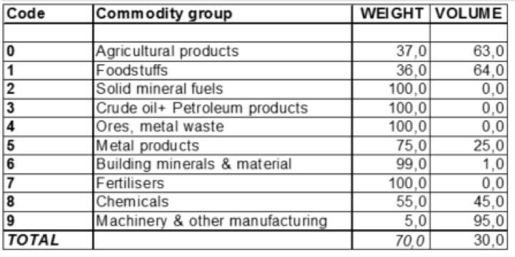
- Both w/ Commodity-dependent probabilities -> defines Weight-only or Volume-only limits subject to the commodity type and an associated probability which is drawn for every tour. This assumes only one commodity is transported per tour. Probabilities are below.
To-Do
Commodity compatibility
The following specifications for commodity compatibility in the same vehicle have been drafted:
- Live animals or animal products
- Vegetable products
- Food
- Beverage or Tobacco
- Chemicals, rubber or plastics
- Clothing or textiles
- Machinery, appliances, and mechanical parts
- Minerals, ore, stone, cement, ceramics or glass
- Wood, paper or straw products
- Metals or articles of metal
- Miscellaneous manufactured products
- Vehicles
- Waste or scrap
| 1 | 2 | 3 | 4 | 5 | 6 | 7 | 8 | 9 | 10 | 11 | 12 | 13 | |
|---|---|---|---|---|---|---|---|---|---|---|---|---|---|
| 1 | X | ||||||||||||
| 2 | X | ||||||||||||
| 3 | X | ||||||||||||
| 4 | X | ||||||||||||
| 5 | X | ||||||||||||
| 6 | X | ||||||||||||
| 7 | X | ||||||||||||
| 8 | X | ||||||||||||
| 9 | X | ||||||||||||
| 10 | X | ||||||||||||
| 11 | X | X | X | X | X | X | X | X | |||||
| 12 | X | ||||||||||||
| 13 | X |
User Debug mode specifications
Report on the aggregated output:
- “x records were passed to Carrier Selection and Operations Planning model.”
- “x out of y records were assigned to a vehicle.”