Is History Worth Learning?

Most traders rely on historical price series in their attempt to predict the future price moves. It may be technical analysis and indicators, it may be quantitative trader's momentum strategies, or it may even be some sophisticated machine learning models. There are countless books and research papers on the subject, and once in a while we hear great success stories from a few very lucky traders turning $5K into $1M or some such. However, it appears that it's not particularly easy to replicate such success - or else millions of people would now be very rich.

At the same time, all brokers clearly state in their legal disclaimer that "historical prices are not an indication of future performance". Which, if true, would render all the above strategies completely useless. So, is this just a legal speak, or they actually mean it?

Therefore, the fundamental question is, how much predictive information do historical prices actually have? Let's find out!

Prices, changes, and random variables

Let's start at the very beginning. Say, we have a stock A with its historical price series p(t). While the actual price is ultimately discrete (it changes in ticks, the individual buy/sell transactions), the ticks happen so rapidly (sometimes every microsecond!) that it is convenient to assume that the price is continuous. The absolute price value is often irrelevant, as long as we can afford to buy at least one stock. What's really relevant for us as traders is the relative change of the price: will it grow by 1%, by 10%, or will drop by 50%? And therefore, the really interesting time series is not p(t) itself, but rather the series of the relative changes:

d(t) = (p(t) - p(t-1)) / p(t-1).

In particular, d(t)=0.01 means the price has gone up by 1% since the previous bar, while d(t)=-0.5 means it dropped by 50%.

In the literature, people sometimes use the log-price difference, such as l(t) = log(p(t)) - log(p(t-1)), but for relatively small changes this happens to be about the same as d(t):

log(p(t)) - log(p(t-1)) = log(p(t)/p(t-1)) 
 = log(1 + (p(t) - p(t-1)) / p(t-1))
 =~ (p(t) - p(t-1)) / p(t-1)
 = d(t)

So, to make our live simpler, we just use d(t).

Since the market obviously moves with high degree of randomness, it is reasonable to model d(t) as a series of random variables D(t). Further, to make things simple, we assume that all these variables for each stock have exactly the same probability distribution. Furthermore, although the price is technically discrete, for convenience we assume it's continuous, and therefore, its distribution is characterized by a p.d.f. f(x).

As a side note, f(x) for most of the stocks traded on the major US exchanges is very closely approximated by the Student T distribution with the parameter a=3 (this fact, its derivation and the consequences that follow deserve a separate post, TBD). That is:

f(y) = C * (1 + y^2 / a)^(-(a+1)/2)

where C = 1 / (sqrt(a)*Beta(1/2, a/2)), and x = k*y+m to account for scaling and non-zero mean (since generally stocks tend to grow over long term). However, this fact is not particularly relevant to our discussion below, other than, perhaps, the fact that f(y) is a fat tail distribution with the degree a. That is, the tails of the cumulative distribution function converge to 0 and 1 respectively as polynomials of degree a. In particular, this implies that very large (much larger than, say, 10-MAD) moves are relatively common, as we shall soon see, whereas their probability would be prohibitively low for a Gaussian distribution.

Independent random variables

By definition, a random variable X is independent of Y if f(x | y) = f(x). Therefore, it is sufficient to compare the two distributions in order to test whether two variables are independent.

We can now consider random variables X=D(t) and Y=D(t-k) from the sequence D as defined above, and collect values of d(t) as samples from the distribution of D(t). Now, if we can compute f(x|y) and f(x) from the samples, and then meaningfully compare them for various values of k>0, we'll be able to tell if there is any useful information in the previous samples to predict the value of a future price move.

Recall, that f(x|y) = f(x, y) / f(y), where f(y) for a given value of y is just a normalizing constant, and the residual p.d.f. f(x) can be computed as an integral \int f(x, y) dx. Thus, it is sufficient to construct an approximation of f(x, y) from the available samples.

Sample Distributions

To reduce the sample noise, we construct f(x, y) as a 2D histogram of values (dt(t), dt(t-k)). The integral then becomes a normalized sum over the corresponding buckets, where dx is the width of the bucket (for linear buckets, dx = (x_max - x_min) / N), where N is the number of buckets in each dimension.

Furthermore, we normalize the mean of D(t) to be zero and the volatility to be 1.0. Volatility here is defined as MAD(D) (mean absolute deviation):

MAD(samples) = sum(|s - mean| for s in samples) / #samples

In particular, this allows us to merge the samples from many different stocks with possibly different means and volatility.

In our specific experiment, we used two samples:

• "Daily" set: 20 years (2000 - 2020) worth of daily closing prices from all the stocks traded on major US exchanges: NASDAQ, NYSE and AMEX, including stocks that existed in the past but now delisted (so called "survivorship bias free" dataset), about 36M samples total
• "Minutely" set: about 6 months (Jan - Jun 2020) worth of minutely prices from the same US exchanges, about 150M samples total.

We then used N=100 (so, the 2D histogram has 10K buckets) with a range of values for normalized d(t) [-40..40]. Recall, that this scale is in "MADs" (mean absolute deviations), which for the Gaussian would be 12% larger than the standard deviation. In other words, we are definitely seeing a lot of very large deviations from the mean in the data that shouldn't be possible if the distribution was Gaussian.

We then construct 300 such histograms for the "daily" set for k=[1..300], and 100 histograms for the "minutely" set for k=1..100. Thus, we are setting up the analysis for checking if there is any influence that many bars into the future.

Measure of "sameness"

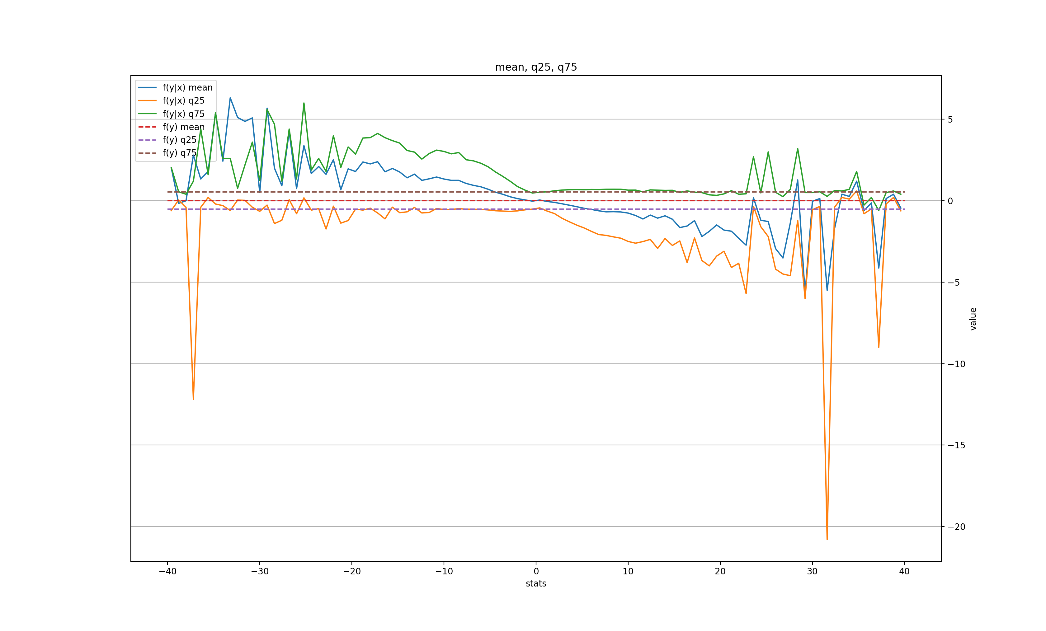
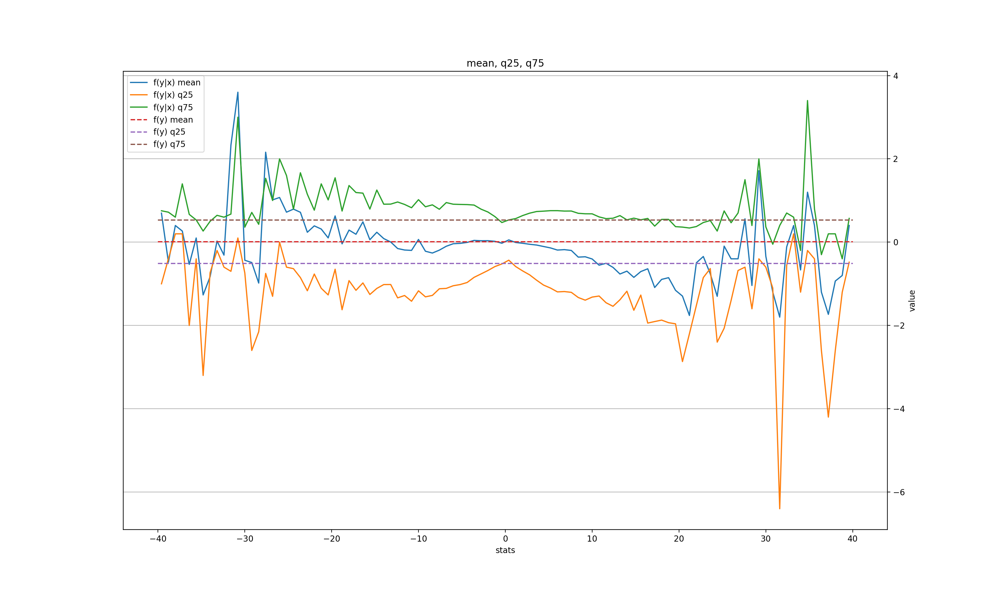
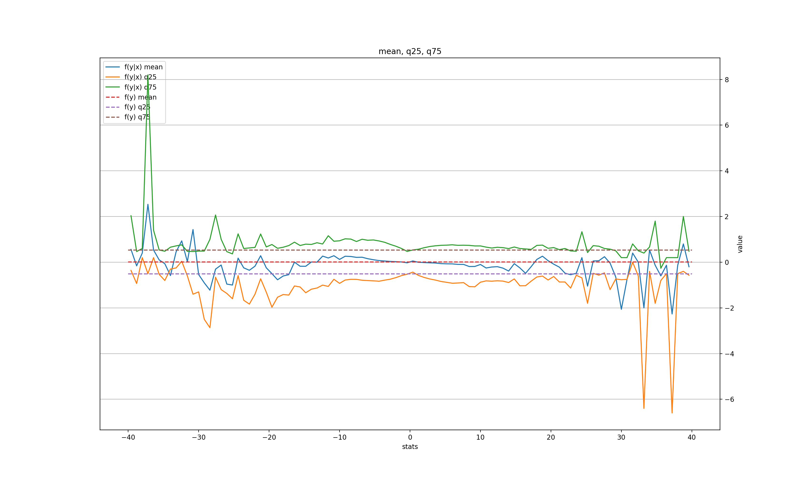
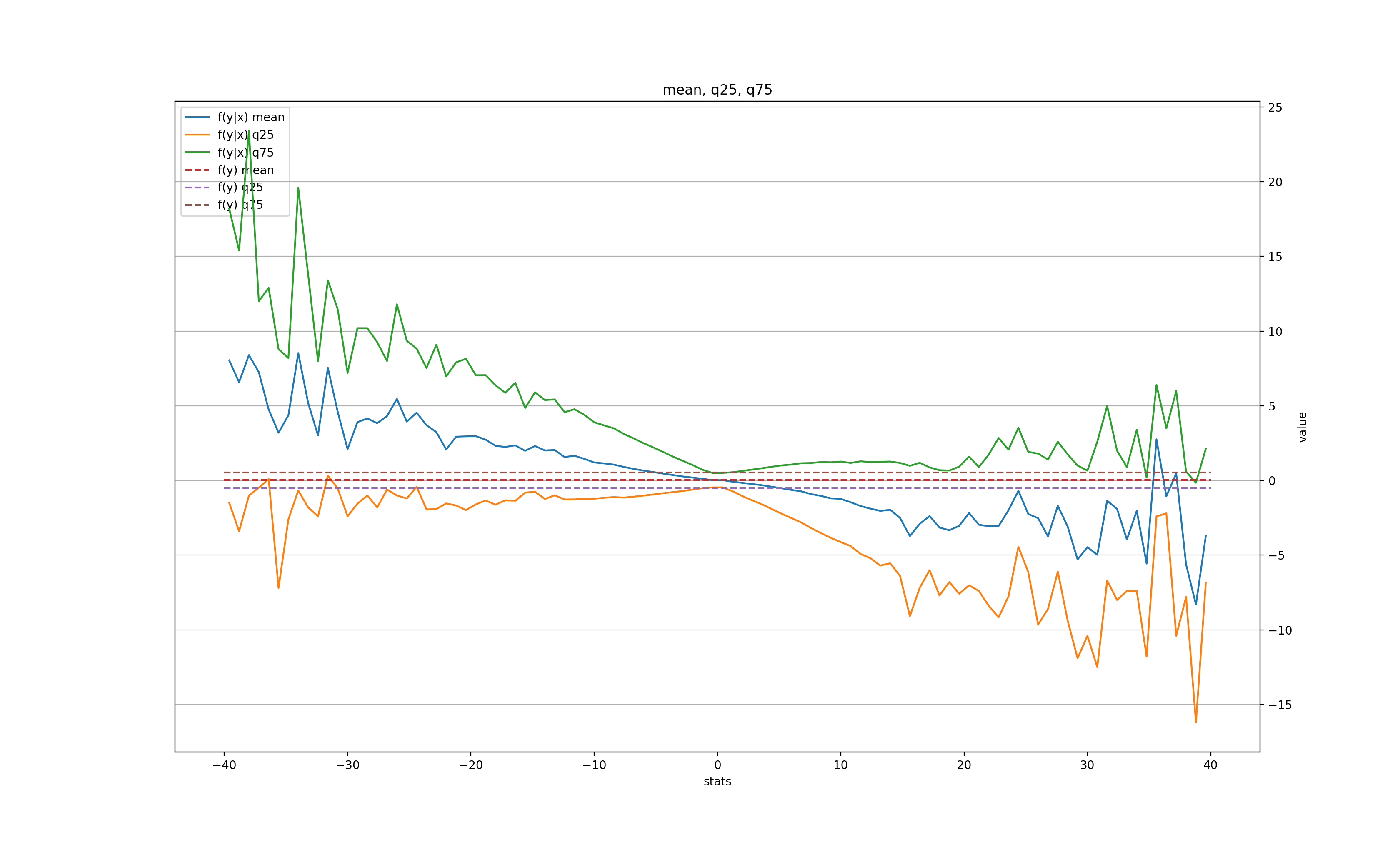
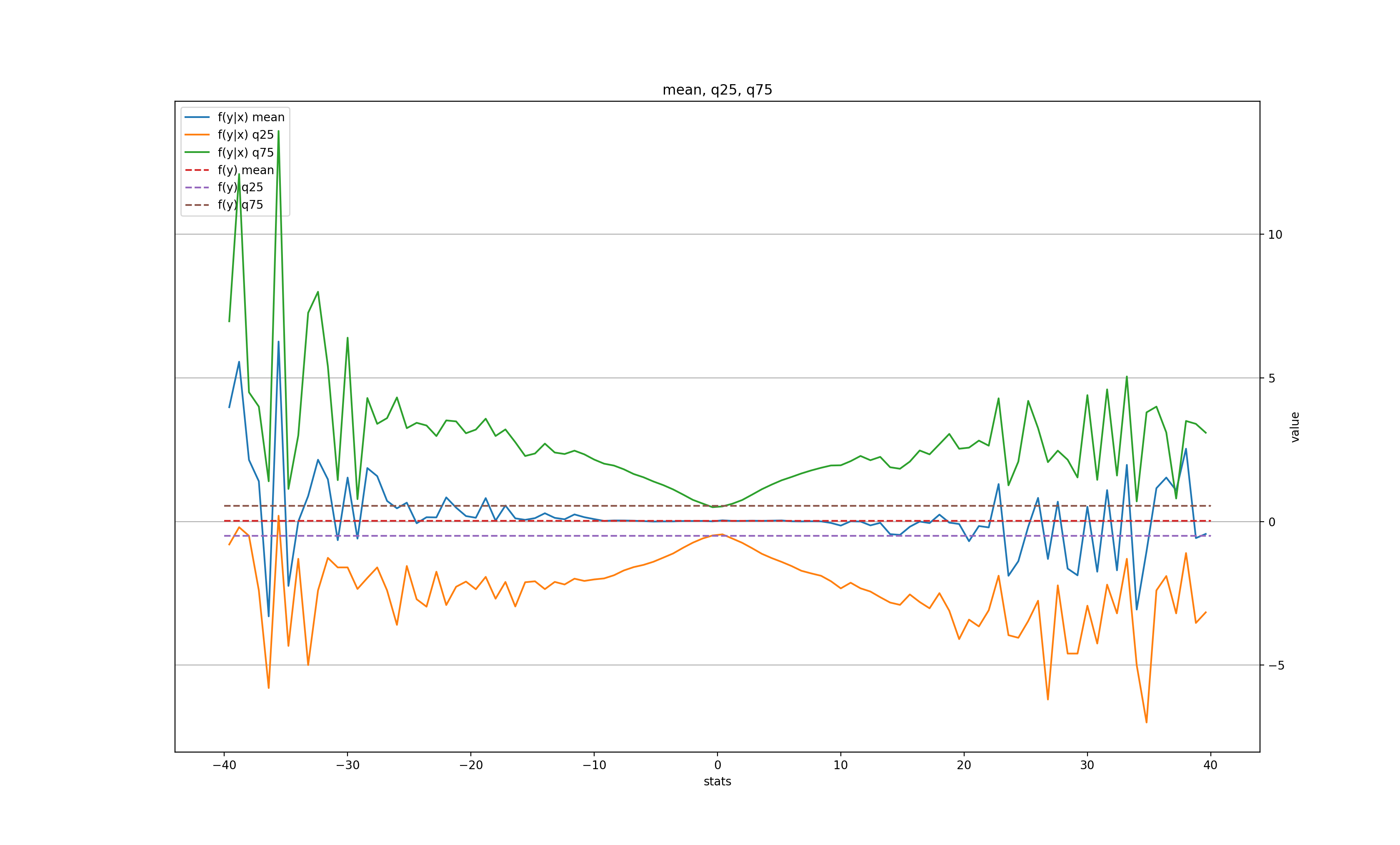
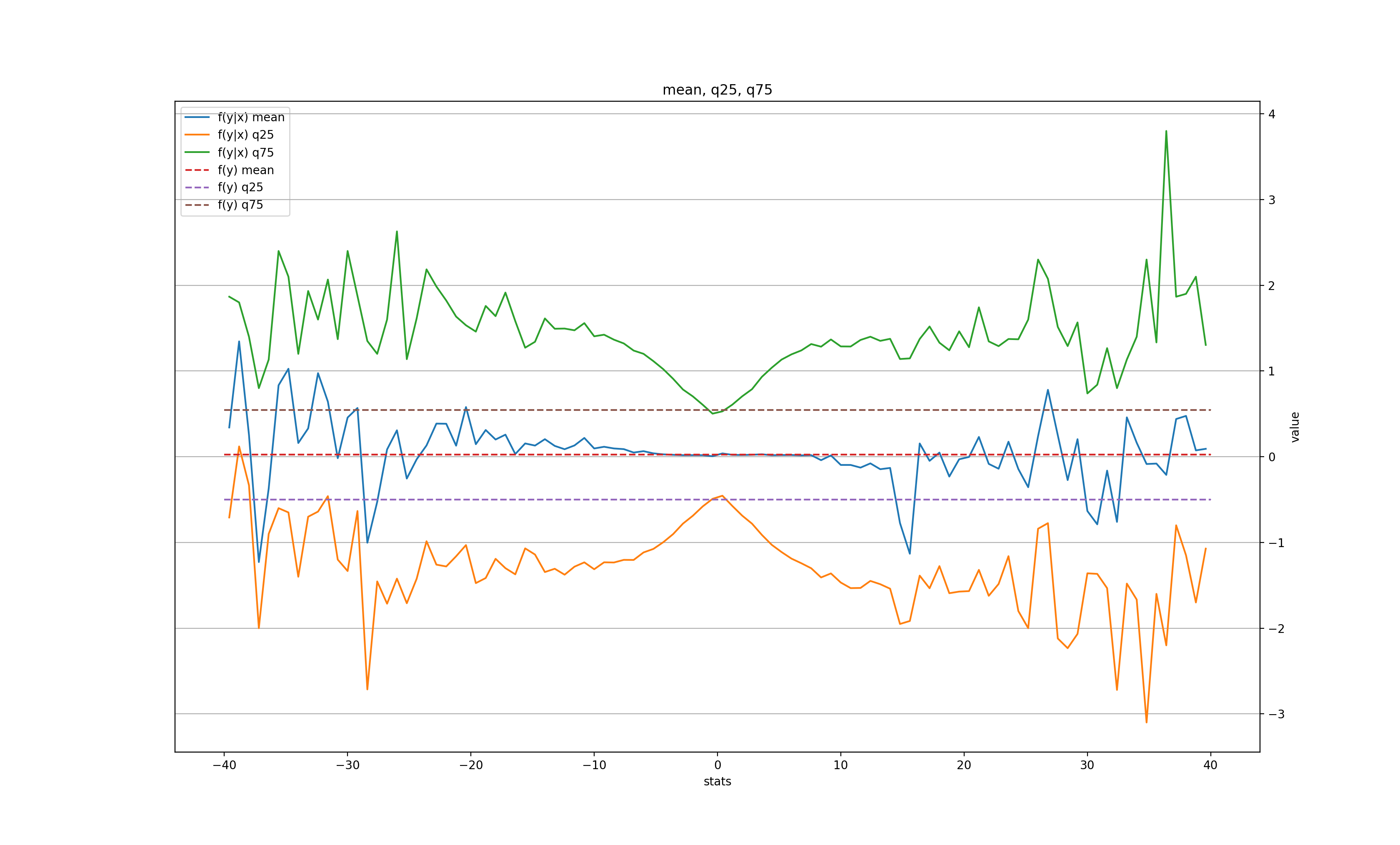
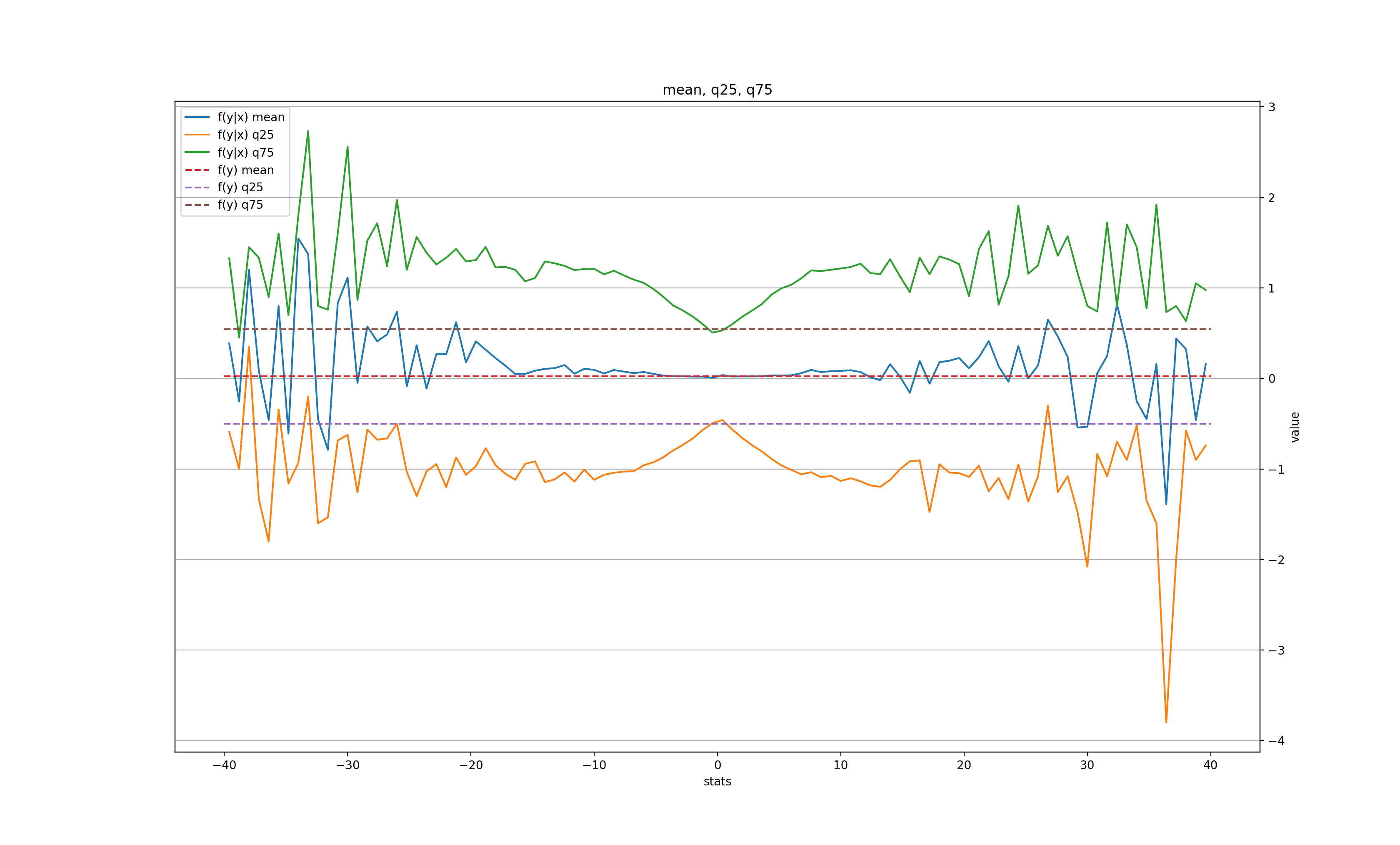
The exact histograms of f(x|y) and f(x) will have a lot of sample noise, especially towards the far ends, and therefore, it is likely counterproductive to apply the more sensitive distance measure Dist[f, g]=max(|f(x)-g(x)|). However, we can look at the important characteristics of the distributions that can give us the idea for their difference, if any: the mean and the 25th and 75th quantiles. Specifically, we'll compute these values for f(x|y) as a function of y, and compare them with the corresponding values for f(x).

Here's how this plot looks for the "daily" dataset with various k:

k = 1:

k = 2:

k = 3:

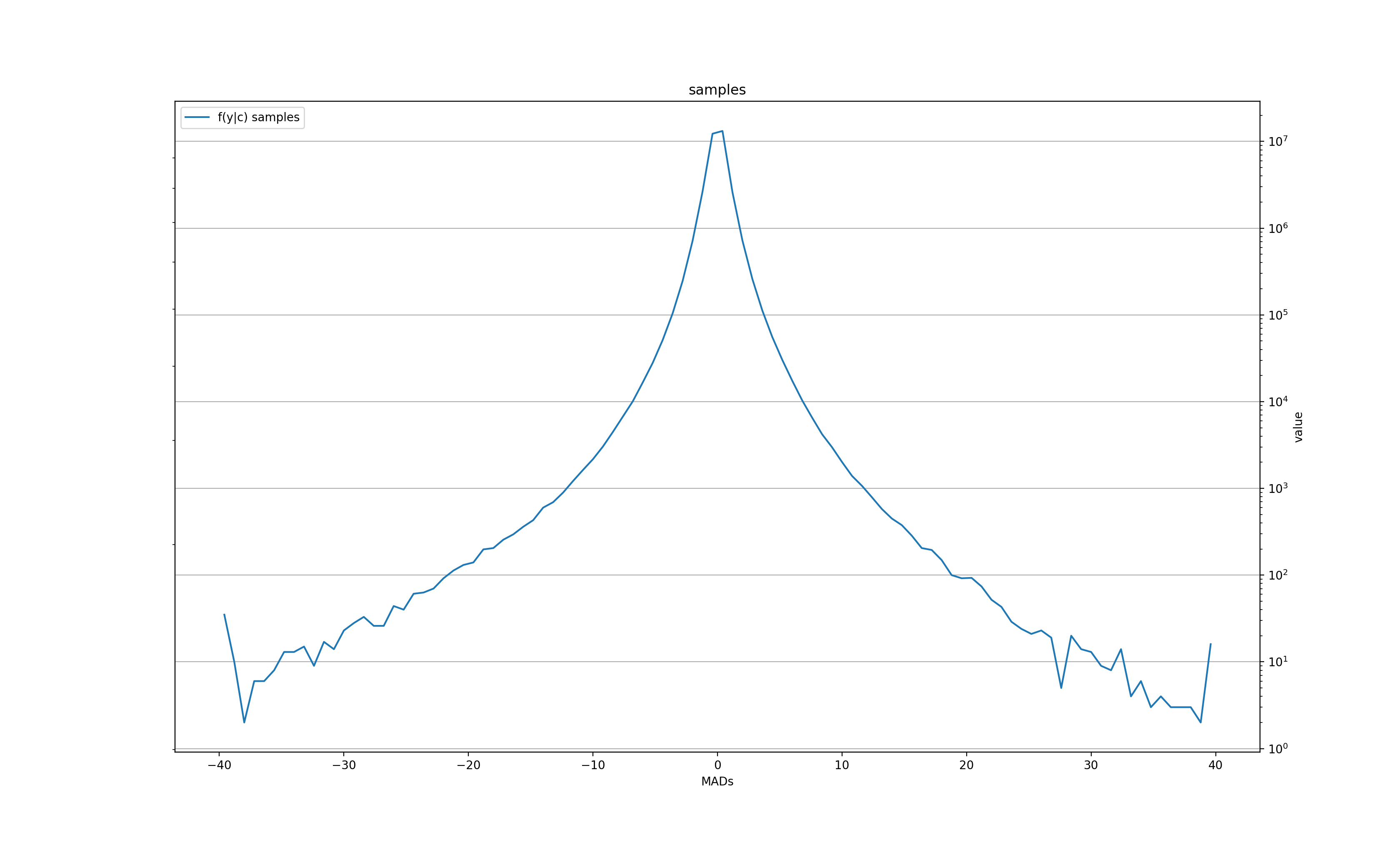
The number of samples for f(x|y) histogram at each quantized value y:

In other words, there is some signal for very large moves (over 3-4 MADs) in the next day (the price tends to roll back slightly), and even a bit in the second day, but after 3 days all is forgotten. There is also a clear tendency for the volatility to grow after a large change, but also only for the next couple of days before settling back to normal.

What about the minutely data?

k = 1:

k = 2:

k = 10:

k = 20:

The corresponding sample size for f(x|y) at each y:

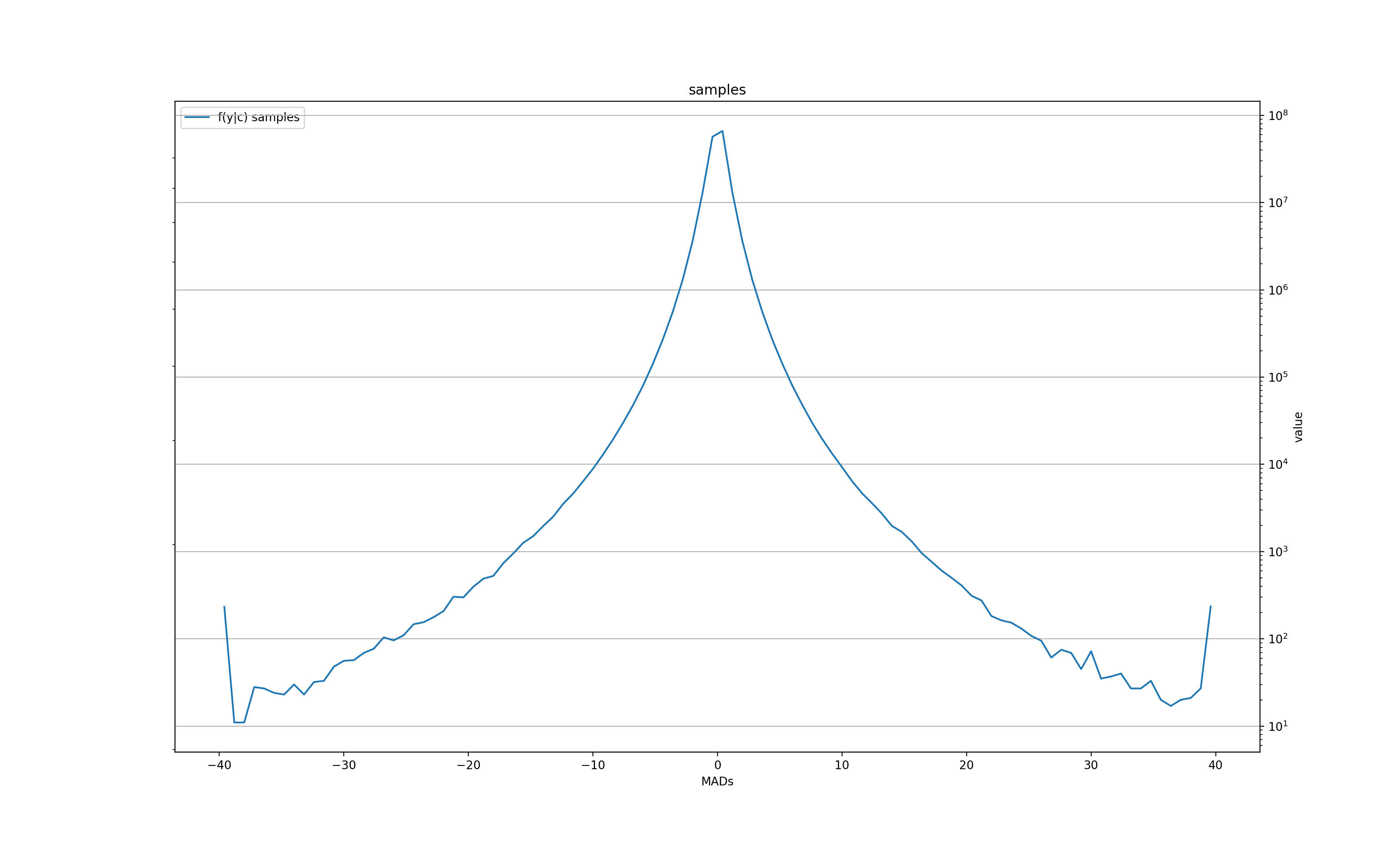
Unlike the daily data, the "memory" of the large move only lasts for 1 minute in the mean, but is still there 20 minutes later in the volatility.

In both "daily" and "minutely" datasets, there is a clear signal for the next bar, but only after a very large (and therefore, rare) price move, with a tendency to roll back towards its previous value. This somewhat validates the "breakout" trading strategy, when a trader waits for an unusually large move of the price and places a bet for the price to come back. In this case, we'd wait for, let's say, a 10-MAD breakout either in daily or on minutely series, and immediately place a bet for the next bar that the price will recoil, even if only slightly (for a 10-MAD breakout the average recoil is about 1 MAD in daily and 2 MADs in minutely).

There is, however, a catch: these tendencies are averages over thousands of samples. In fact, the mean in both datasets begins to deteriorate below 1000 samples (corresponding to 10 MADs in daily and 15 MADs in minutely graphs). Making thousand transactions takes a very long time, especially in daily trading, and lots of money in transaction fees, which likely makes this strategy not practical.

And for the bulk of the smaller moves (under 2 MADs, ~95% of all price moves), there doesn't seem to be any signal at all, at least not for the mean and the width of the distribution. Which also means that most other momentum-based strategies have little to no basis for working.

Possible shortcomings of the approach

These 3 metrics can't imply the equality of the distributions...

It may indeed be useful to apply a more thorough distance metric to the distributions, at least to the range where they both have enough samples for a statistically significant result. This would indeed show a better measure of (in)dependence, albeit without the useful insights that the above 3 metrics provide. I'll update this section if I implement it in the future.

My hunch, however, is that the shape of the conditional distribution remains roughly the same as the residual one, and thus these metrics should be rather good indicators of "sameness" of the distributions. In any case, trading most often relies on the mean, since that's what ends up contributing to the equity curve across many transactions, and therefore, even if the distributions differ, the same mean often means there is no game.

The histogram is too coarse near zero. Maybe we just can't resolve something interesting there?

This is indeed a valid point, and I'm in the process of updating the histogram with exponentially growing buckets to improve the resolution near zero, where the bulk of the action happens. I wouldn't hold my breath though, since the mean will very likely stay close to zero even at higher resolution, implying no useful information for personal enrichment.

But, maybe, we should look at several affected bars?

It's true that we've only looked at a single bar affecting another single bar in the future. Can it happen that any given bar indeed doesn't influence any other given bar most of the time, but it still influences the average price change over multiple bars in the future?

Well, recall that what we're looking at are already averages across many thousands or even millions of samples. My admittedly hand-wavy argument is that, if a bar would influence a price move across multiple bars, but not at any specific bar in that sequence, it only means that the growth (or drop) is randomly spread out across these many bars. Which, in turn, means that averaging over many such sequences will yield a small but steady growth (or drop, respectively) for each such bar. Thus, looking at a single bar should be sufficient.

OK, but maybe it's several bars affecting future bars then?

If we are talking about several past bars affecting several future bars, we are really talking about single bars at larger time scales, e.g. weekly or monthly bars. It also implies that the stocks have some "natural" frequency or time scale at which something repeats, but in between there is mostly noise. This is why I looked at two vastly different time scales - daily and minutely, just to discover that they look essentially identical, somewhat affecting the very next bar and not much else (besides the volatility). This suggests that other time scales are not likely to look materially different.

In fact, in my other experiments with long term investments I've used quarterly bars (3 months long), and the result is mostly the same - no useful predictive power. And one would think that at these scales we should be able to tell truly successful businesses from flops. But alas, no - even a really good multi-year growth track still has no predictive power for the next year...

But, but... this is too simple. Maybe the patterns are more complex?

Maybe, and that's why a better distance measure between f(x|y) and f(x) is in order. However, looking at the distributions directly suggests that they don't significantly change the shape other than increasing volatility. Hence, there is hardly any pattern other than just that - increased volatility after a large move.

Given that (useless) volatility increase persists longer than the (useful) change in the mean, we may consider re-normalizing f(x|y) to 1-MAD width before comparing to f(x), so we can catch any material changes in the shape. It's an idea for the future.

As to more complex patterns spanning multiple bars (like support / resistance, divergent peaks, "head and shoulders", etc.) - I'd be very surprised to see them in the stocks. Part of the reason is the same as with multiple bars above: such patterns should average out into some dependency. In particular, into some dependency across multiple bars (which we don't observe). And another part is that there is simply no good reason for such patterns to sustain themselves. Chances are, lots of smart people with ML models and lots of (institutional) cash are probably catching hints of such patterns that occasionally emerge and trading them out of existence.

So, there is no hope for a generic strategy. But maybe each stock may still have its own patterns?

Possibly. However, each individual stock doesn't have enough data, especially daily, to confirm those patterns in any statistically significant way. As we've seen above, one needs around 1000 samples to reduce the noise is the mean to acceptable levels, which is about 4 years of daily data, assuming that the pattern happens every day. But successful companies tend to evolve faster than that (or they wouldn't grow), and by the time a pattern emerges in the historical data, it might already be gone from the future trades.

Similarly, minutely data contain only 450 samples in a day, and at this frequency each day often looks very different from the next.

This is one of the problems with the fat tail distributions: they require a lot more samples to show convergence compared to e.g. Gaussian, and the available sample size is often insufficient.

Conclusions

While there is a tiny bit of predictive information in the historical prices, the brokers and their lawyers are mostly right - history tells us essentially diddly squat about future performance. The market is indeed rather efficient, most likely thanks to the millions of traders who diligently place their bets in the biggest casino in the World called the Exchange.