WW II weather data and Gaussian processes - sedgewickmm18/mmfunctions GitHub Wiki
This time I'm trying to predict max temperature from the minimal temperature and precipitation. Notebook is found here
Note that Gaussian processes require a lot of computational power for a large set of observation points - it's complexity is O ( n 3 )
-
Gaussian Processes for little data starts with explaining OLS (ordinary least square) across a parameter space (parameters of a polynomial). Then he moves to his main subject, the non-parametric GP and explains the mathematical background. Furthermore he shows how to implement the covariance matrix based on the radial basis kernel.
-
Gaussian Processes are not so fancy is a more lightweight introduction to the subject.
-
Gaussian Process and Big Data deals with scaling Gaussian Processes for big data with lots of observation points.
-
Visual Exploration of Gaussian Processes is the most aesthetically appealing article.
-
Tutorial with lots of examples how to plot data.
-
My favorite for the mathematical background A copy of it is found in this github repo here
As usual we kick of the notebook by importing libraries we need.
import pandas as pd
import numpy as np
import matplotlib.pyplot as plt
import seaborn as seabornInstance
from sklearn.model_selection import train_test_split
from sklearn.linear_model import LinearRegression
from sklearn import gaussian_process
from sklearn.gaussian_process import GaussianProcessRegressor
from sklearn.gaussian_process.kernels import RBF, WhiteKernel, ExpSineSquared, ConstantKernel as C
from sklearn.preprocessing import StandardScaler
from sklearn.model_selection import ShuffleSplit
import sklearn.decomposition
import sklearn.metrics
%matplotlib inline
Let's read the weather data
dataset = pd.read_csv('./Weather.csv', dtype={"Snowfall":object, "PoorWeather":object, "SNF": object, "TSHDSBRSGF":object})
and fix precipitation data we need later
dataset['Precip'] = pd.to_numeric(dataset['Precip'], errors='coerce')
dataset = dataset.fillna(0)
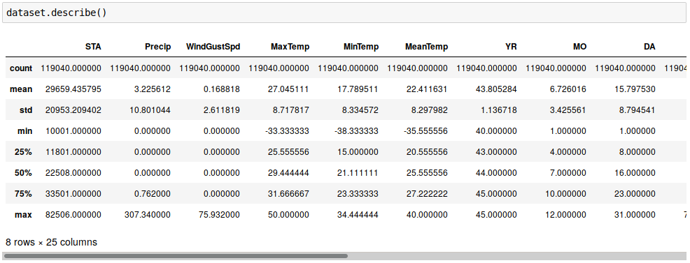
dataset.shape
The last statement should return (119040, 31)
We have now the following data
that we have to 'massage' a bit
#prepare data, sort by minimal temperature and turn X,y into a function
df = dataset[['MinTemp','Precip','MaxTemp']]
#just take the first 1000 values - the full dataset takes way too much memory
X = df.values[:,0:-1]  # features MinTemp & Precip
y = df.values[:,2]  # target
X_train = df.head(1000).values[:,0:-1]
y_train = df.head(1000).values[:,2]
#X_train, X_test, y_train, y_test = train_test_split(X, y, test_size=0.2)
before we dive right into Gaussian Processes.
np.random.seed(1)

#Predict max temp from min temp and precipitation
kernel = C(1.0, (1e-3, 1e3)) * RBF(10, (1e-2, 1e2))

gp = GaussianProcessRegressor(kernel=kernel, n_restarts_optimizer=9)

gp.fit(X_train, y_train)

print (gp.score(X_train, y_train))

y_pred, sigma = gp.predict(X, return_std=True)

# Back to a dataframe
dfnew = pd.DataFrame({'MinTemp': X[:,0], 'Precip': X[:,1], 'MaxTemp': y[:], 'MaxPred': y_pred})

# and predict for the training data only
y_predT, sigma = gp.predict(X_train, return_std=True)
Sigma is 0.5901525736283517 so our R2 score is rather mediocre
Plotting observations and predictions for training data with
# Gaussian doesn't like values below 0 !!!
plt.figure(figsize=[10,7])

plt.plot(X_train[:,0], y_train, 'r.', markersize=10, label='MinTemp')
plt.plot(X_train[:,1], y_train, 'g.', markersize=10, label='Precipitation')
plt.plot(X_train[:,0], y_predT, 'b-', label='Prediction')
plt.plot(X_train[:,1], y_train, 'y-', markersize=10, label='Prediction2')
#plt.fill(np.concatenate([X, X[::-1]]),
#         np.concatenate([y_pred - 1.9600 * sigma,
#                       (y_pred + 1.9600 * sigma)[::-1]]),
#         alpha=.5, fc='b', ec='None')
#         alpha=.5, fc='b', ec='None', label='95% confidence interval')
plt.xlabel('$MinTemp$')
plt.ylabel('$MaxTemp$')
plt.ylim(-10, 35)
plt.xlim(-10, 35)
plt.legend(loc='upper right')
yields
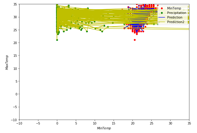
Let's see how good we predict non-training data with
df1 = dfnew.head(30) + 40 # lift by 40 for strictly positive numbers
df1.plot(kind='bar',figsize=(16,10))
plt.grid(which='major', linestyle='-', linewidth='0.5', color='green')
plt.grid(which='minor', linestyle=':', linewidth='0.5', color='black')
plt.show()
to generate the following plot.
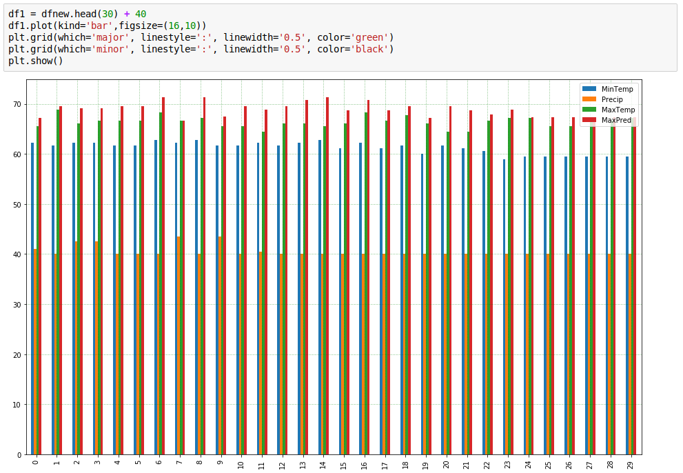
Last little plot shows we're doing so lala
Linear regression is better ;-)
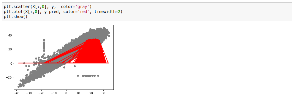
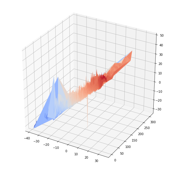
3-d plotting of MinTemp, Precipitation and MaxTemp exhibits a rough linear relationship between the 2 temperature values (as expected).
from matplotlib import cm
from mpl_toolkits.mplot3d import axes3d
fig = plt.figure(figsize=(10,10))
ax = fig.add_subplot(111, projection='3d')
ax.plot_trisurf(df['MinTemp'], df['Precip'],df['MaxTemp'], cmap = cm.coolwarm, linewidth=0.2)
plt.show
After cleansing data and removing rows where MinTemp > MaxTemp with df = df1[~(df1['MinTemp'] > df1['MaxTemp'])] # strip rows where MinTemp > MaxTemp and taking the first 3000 elements as training data results are slightly better.
BTW, fitting (training) took quite long time, i.e. ~30 mins - complexity of O(n3) shows off. As a result training, especially training with multiple parameters, for example different kernels to find the best one via cross validation, is not the kind of function you want to run synchronously in your pipeline.
The mmfunction module also contains a GaussianProcess subclass of BaseEstimatorFunction. Run ./register.py test to execute a rather run with over a one-dimensional feature space to generate column5 with its predictions - it's test case number 4. It's just there to show the plain "mechanics".