Splittingfunc - s-schneider/frospy GitHub Wiki
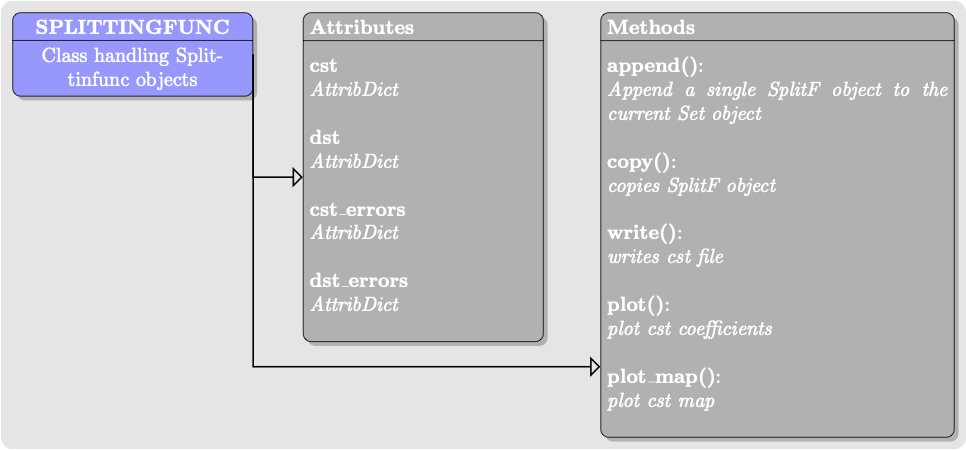
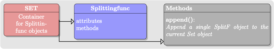
Splitting functions are depth weighted averages of how a particular mode sees the Earth. This can be found in the two classes splittingfunc and Set. Set are list-like objects which contain multiple splittingfunc objects. The splittingfunc object contains splitting function observations (cst and dst) and their associated errors (cst_errors and dst_errors), both of which are dict-like objects.
To import the cst coefficients and dst coefficients of mode from Schneider & Deuss, 2021 (SAS), you can use the following lines of code, which creates a splittingfunc object, containing only the mode
from frospy import load
SF = load(modes='0T4', format='SAS')
>>> print(SF.cst)
AttribDict({'0T4': AttribDict({'0': array([ 0.47672686]),
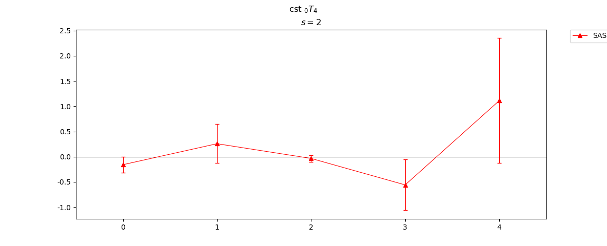
'2': array([-0.15809828, 0.25792417, -0.03396468, -0.55866814, 1.11150587]),
'4': array([-0.08044234, -0.32076186, -0.57898396, -0.31278956, 0.06608175, 0.20384744, 0.09049329, 0.47444671, 0.44629607]),
'6': array([ 0.03940144, -0.37996399, -0.17887443, 0.62207186, 0.16380437, 0.12194022, -0.30844843, 0.11956441, 0.50576258, 0.43592972, 0.0931734 , -0.45840219, 0.17707771]),
'8': array([ 0.0748193 , 0.19456637, -0.18266548, -0.89382917, -0.11207749, -0.06527079, -0.30490938, 0.21710126, -0.19156709, 0.37253278, 0.02100956, -0.16518703, -0.34745032, -0.18519123, 0.13239613, 0.48933321, -0.12593114])})})
>>> print(SF.cst_errors)
AttribDict({'0T4': AttribDict({'0': QuantityError({'uncertainty': array([ 0.71299052]), 'lower_uncertainty': array([ 0.47539312]), 'upper_uncertainty': array([ 0.71299052]), 'confidence_level': [95.0]}), '2': QuantityError({'uncertainty': array([ 0.15941604, 0.38631237, 0.06663173, 0.50420862, 1.23942459]), 'lower_uncertainty': array([-0.15941604, 0.26777515, -0.06547331, -0.50420862, 1.12589622]), 'upper_uncertainty': array([-0.05572271, 0.38631237, 0.03063844, -0.16643572, 1.23942459]), 'confidence_level': [95.0, 95.0, 95.0, 95.0, 95.0]}), '4': QuantityError({'uncertainty': array([ 0.14030738, 0.31022584, 0.51174945, 0.23922871, 0.22869188,
0.34241855, 0.2833941 , 0.68715996, 0.62215787]), 'lower_uncertainty': array([ 0.02156383, -0.31022584, -0.51174945, -0.23922871, 0.11356808,
0.18577658, 0.02785176, 0.53645569, 0.49656481]), 'upper_uncertainty': array([ 0.14030738, -0.16456737, -0.20462315, 0.03772717, 0.22869188,
0.34241855, 0.2833941 , 0.68715996, 0.62215787]), 'confidence_level': [95.0, 95.0, 95.0, 95.0, 95.0, 95.0, 95.0, 95.0, 95.0]}), '6': QuantityError({'uncertainty': array([ 0.26685357, 0.3951872 , 0.25453708, 0.65174228, 0.39073661,
0.19761023, 0.35137215, 0.2322652 , 0.65079212, 0.63254231,
0.28287294, 0.37903097, 0.22602686]), 'lower_uncertainty': array([ 0.04344824, -0.3951872 , -0.11824709, 0.56947601, 0.16539924,
0.02894482, -0.35137215, 0.06430334, 0.47687063, 0.43769524,
0.14243177, -0.37903097, 0.09140169]), 'upper_uncertainty': array([ 0.26685357, -0.11443686, 0.25453708, 0.65174228, 0.39073661,
0.19761023, -0.18232043, 0.2322652 , 0.65079212, 0.63254231,
0.28287294, -0.19943219, 0.22602686]), 'confidence_level': [95.0, 95.0, 95.0, 95.0, 95.0, 95.0, 95.0, 95.0, 95.0, 95.0, 95.0, 95.0, 95.0]}), '8': QuantityError({'uncertainty': array([ 0.26919296, 0.22600827, 0.27850601, 0.80438906, 0.14245975,
0.15165392, 0.24678777, 0.44948107, 0.23560841, 0.43672037,
0.27404281, 0.15101939, 0.38552982, 0.19909045, 0.29139024,
0.57979995, 0.13707828]), 'lower_uncertainty': array([ 0.08030873, 0.12784341, -0.15716741, -0.80438906, -0.14245975,
0.0010737 , -0.24678777, 0.20104265, -0.23560841, 0.33534285,
0.10147628, -0.15101939, -0.38552982, -0.19909045, 0.09126286,
0.52150232, -0.06196259]), 'upper_uncertainty': array([ 0.26919296, 0.22600827, 0.27850601, -0.70023715, 0.02468726,
0.15165392, 0.00445831, 0.44948107, -0.00701666, 0.43672037,
0.27404281, -0.01944483, -0.16051912, -0.0525703 , 0.29139024,
0.57979995, 0.13707828]), 'confidence_level': [95.0, 95.0, 95.0, 95.0, 95.0, 95.0, 95.0, 95.0, 95.0, 95.0, 95.0, 95.0, 95.0, 95.0, 95.0, 95.0, 95.0]})})})
>>> print(SF.dst)
AttribDict({'0T4': AttribDict({'0': array([-0.83529902])})})
>>> print(SF.dst_errors)
AttribDict({'0T4': AttribDict({'0': QuantityError({'uncertainty': array([ 0.8114475]), 'lower_uncertainty': array([-0.8114475]), 'upper_uncertainty': array([-0.76121503]), 'confidence_level': [95.0]})})})
To access a particular mode and degree type (Both the mode and degree identifiers are strings)
>>> print(SF.cst["0T4"]['2'])
array([-0.15809828,  0.25792417, -0.03396468, -0.55866814,  1.11150587])
>>> print(SF.cst_errors["0T4"]['2'])
QuantityError({'uncertainty': array([ 0.15941604,  0.38631237,  0.06663173,  0.50420862,  1.23942459]), 'lower_uncertainty': array([-0.15941604,  0.26777515, -0.06547331, -0.50420862,  1.12589622]), 'upper_uncertainty': array([-0.05572271,  0.38631237,  0.03063844, -0.16643572,  1.23942459]), 'confidence_level': [95.0, 95.0, 95.0, 95.0, 95.0]})
To obtain the center frequency and Q of the mode computer from the zero degree coefficients use
>>> print(SF.get_fQ(mode_name="0T4"))
((array([ 765.79448216]),
  array([ 0.20113091]),
  array([ 0.20113091]),
  array([ 0.13410592])),
 (array([ 265.54500343]),
  array([ 32.50598719]),
  array([ 22.59540067]),
  array([ 32.50598719])))
which outputs (center freq, center freq err, center freq upper error, center freq lower error) and (Q, Q error, Q upper error, Q lower error)
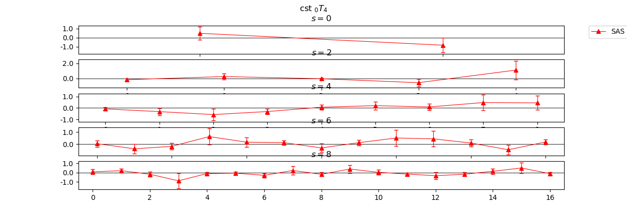
To plot the splitting function coefficients together with their corresponding uncertainties per degree
SF.plot()
To plot the associated splitting function map
SF.plot_map()
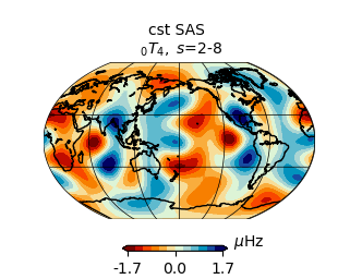
The minimum and maximum degree plotted can be indicated for both plots using smin and smax.
SF.plot(smin=2, smax=2)
SF.plot_map(smax=2)
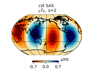 The zero degree contribution (
s=0) is never plotted in plot_map
To write the coefficients of a mode to an external file use (the default format is pickle)
SF.write(filename=modes.out, format="dat")

0.47672686
-0.835299015
-0.15809828
0.257924169
-0.0339646786
-0.558668137
1.11150587
...
The first line of the file contains the c00 coefficient, and second line of the file the d00 coefficient. All s>0coefficients are written after the second line.
To import a Set of modes use
from frospy import load
from frospy.plot.branch import branch
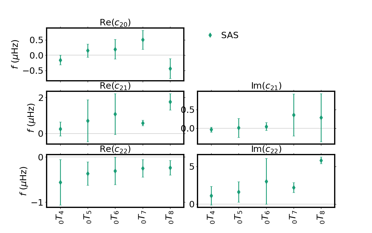
SF = load(format='SAS', modes=['0T4', '0T5', '0T6', '0T7', '0T8'], return_set=True)
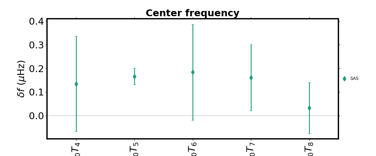
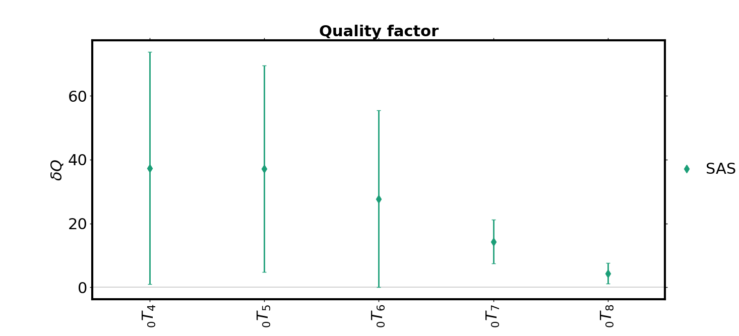
This modes can be plotted as a branch. To plot the center frequency and Q branch use
branch(SF_in=SF, degree=0, plot_f_center=True, mode='t', n=0)
plt.show()
branch(SF_in=SF, degree=0, plot_Q=True)
To plot the degree two use
branch(SF_in=SF, degree=2, mode='t', n=0)
plt.show()
To add additional splitting functions to the Set use
SF += load(modes='0T9', format='SAS')
SF.append(load(modes='0T10', format='SAS'))
>>> print(SF)
7 SplittingFunc(s) in Set:
SAS with cst/dst for:  0T4
SAS with cst/dst for:  0T5
SAS with cst/dst for:  0T6
SAS with cst/dst for:  0T7
SAS with cst/dst for:  0T8
SAS with cst/dst for:  0T9
SAS with cst/dst for:  0T10
To write the Set of modes to an external file called cst-coef.dat
from frospy.core.splittingfunc.write import write
write(SF)
which will write a cst file, and will order the modes in the same way as in the input file. An explanation of the format of the file is given in the file itself.