Spectrum - s-schneider/frospy GitHub Wiki

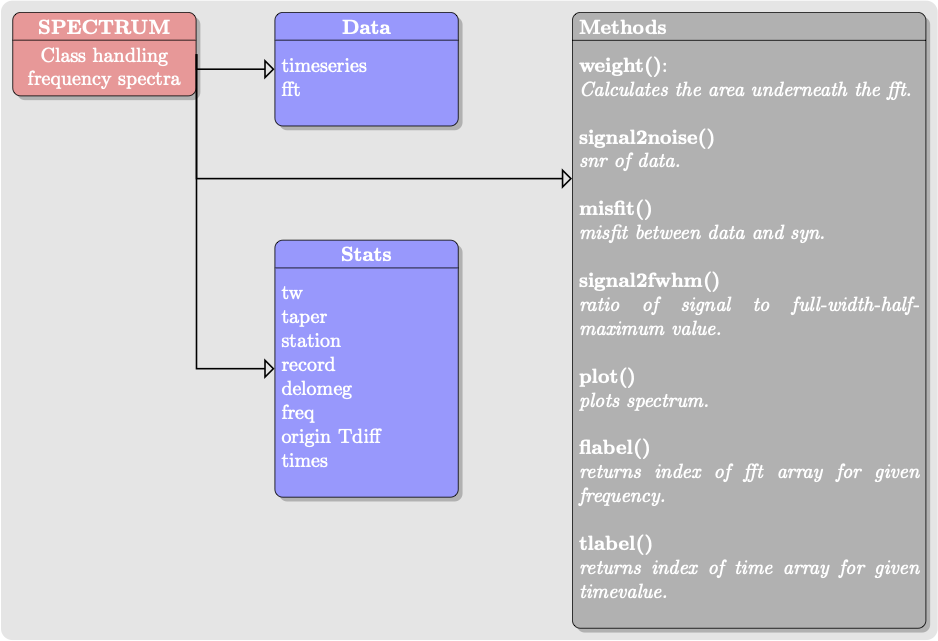
The Spectrum class handles time series data and performs the fast Fourier Transform to obtain the frequency spectrum. Then it is straightforward to plot the spectra, as this example demonstrates:

>>> from obspy.core import read
>>> from frospy.core import Spectrum

# Replace /PATH/TO/REPO with your own frospy repository location
>>> st = read('/PATH/TO/REPO/frospy/data/examples/031111B.ahx')
>>> tr = st[0]
# Time window
>>> hours_start = 5
>>> hours_end = 50
>>> S = Spectrum(tr, hours_start, hours_end)
>>> print(S.stats)
ADO | VHZ | 5.0-50.0 hrs
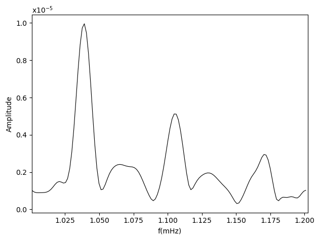
# Frequency window
>>> freq_start = 1.0
>>> freq_end = 1.2
>>> S.plot(freq_start, freq_end, show=True)

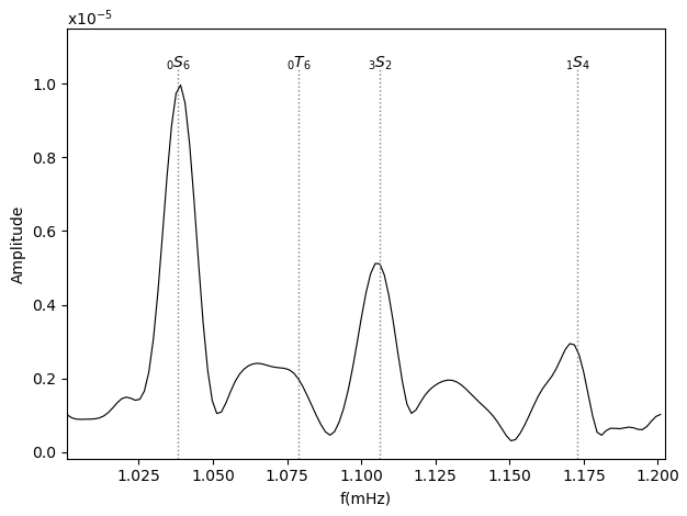
In the following example we include mode lines located at the center frequency of the modes within the frequency window. The center frequencies are read from the mode catalogue.

>>> from frospy.core import Spectrum
>>> from frospy.core.spectrum.plot import plot_modes
>>> from frospy.core.modes import read as read_modes

>>> from obspy.core import read
>>> import matplotlib.pyplot as plt

# Replace /PATH/TO/REPO with your own frospy repository location
>>> st = read('/PATH/TO/REPO/frospy/data/examples/031111B.ahx')
>>> tr = st[0]
>>> hours_start = 5
>>> hours_end = 50
>>> freq_start = 1.0
>>> freq_end = 1.2
>>> S = Spectrum(tr, hours_start, hours_end)

# Reading the mode catalog
>>> modes = read_modes()

>>> fig, ax = plt.subplots()
# To plot the amplitude spectrum for the given frequency window
>>> S.plot(freq_start, freq_end, ax=ax, part='Amplitude')
# Adding normal mode frequenies to the plot
>>> plot_modes(S, freq_start, freq_end, modes, ax)
>>> plt.show()

sourcecode